Time series analysis and forecasting. Time series forecasting methods. Expert forecasting methods

The previous three notes described regression models that predict response from the values ​​of explanatory variables. In this note, we will show how to use these models and other statistical methods to analyze data collected over successive time intervals. According to the characteristics of each company mentioned in the scenario, we will consider three alternative approaches to time series analysis.

The material will be illustrated with a through example: revenue forecasting for three companies. Imagine that you are an analyst at a large financial company. To assess the investment prospects of your clients, you need to predict the returns of three companies. To do this, you collected data on three companies of interest to you - Eastman Kodak, Cabot Corporation and Wal-Mart. Since companies differ in the type of business activity, each time series has its own unique characteristics. Therefore, it is necessary to use different models for forecasting. How to choose the best forecasting model for each company? How to evaluate investment prospects based on forecasting results?

The discussion begins with an analysis of annual data. Two methods of smoothing such data are demonstrated: moving average and exponential smoothing. It then demonstrates the procedure for calculating the trend using the least squares method and more advanced forecasting methods. Finally, these models are extended to time series based on monthly or quarterly data.

Download note in or format, examples in format

Forecasting in business

Insofar as economic conditions change over time, managers must anticipate the impact these changes will have on their company. One of the methods to ensure accurate planning is forecasting. Despite the large number of developed methods, they all pursue the same goal - to predict events that will occur in the future in order to take them into account when developing plans and strategies for the company's development.

Modern society is constantly experiencing the need for forecasting. For example, in order to develop the right policy, members of the government must forecast the levels of unemployment, inflation, industrial production, income tax individuals and corporations. To determine equipment and staffing requirements, airline directors must correctly predict air traffic volumes. In order to create enough space in the hostel, administrators of colleges or universities want to know how many students will enter their institution next year.

There are two generally accepted approaches to forecasting: qualitative and quantitative. Qualitative forecasting methods are especially important if quantitative data are not available to the researcher. As a rule, these methods are highly subjective. If data on the history of the object of study is available to the statistician, quantitative forecasting methods should be used. These methods allow you to predict the state of an object in the future based on data about its past. Quantitative forecasting methods fall into two categories: time series analysis and cause-and-effect analysis methods.

time series is a set of numerical data obtained over consecutive periods of time. The time series analysis method allows you to predict the value of a numerical variable based on its past and present values. For example, daily stock quotes on the New York stock exchange form a time series. Another example of a time series is the monthly index values consumer prices, quarterly gross domestic product and annual income from the sales of a company.

Cause-and-effect analysis methods allow you to determine what factors affect the values ​​of the predicted variable. These include methods of multiple regression analysis with lagging variables, econometric modeling, analysis of leading indicators, methods of analysis of diffusion indices and other economic indicators. We will only talk about forecasting methods based on time analysis. s x rows.

Components of the classical multiplicative time model s x rows

The main assumption underlying the analysis of time series is as follows: the factors that affect the object under study in the present and the past will also affect it in the future. Thus, the main goals of time series analysis are to identify and highlight the factors that are important for forecasting. To achieve this goal, many mathematical models have been developed to study the fluctuations of the components included in the time series model. Probably the most common is the classical multiplicative model for yearly, quarterly and monthly data. To demonstrate the classic multiplicative time series model, consider the data on the actual income of the company Wm.Wrigley Jr. Company for the period from 1982 to 2001 (Fig. 1).

Rice. 1. Graph of Wm.Wrigley Jr.'s actual gross income. Company (million dollars in current prices) for the period from 1982 to 2001

As you can see, over the course of 20 years, the actual gross income of the company had an increasing trend. This long-term trend is called a trend. trend is not the only component of the time series. In addition to it, the data has cyclic and irregular components. Cyclical component describes the fluctuation of data up and down, often correlated with business cycles. Its length varies from 2 to 10 years. The intensity, or amplitude, of the cyclic component is also not constant. In some years, the data may be higher than the value predicted by the trend (ie, be near the peak of the cycle), and in other years it may be lower (ie, be at the bottom of the cycle). Any observed data that does not lie on a trend curve and is not subject to a cyclic relationship is called irregular or random components. If data is recorded daily or quarterly, there is an additional component called seasonal. All components of the time series typical for economic applications are shown in fig. 2.

Rice. 2. Factors affecting the time series

The classic multiplicative time series model states that any observed value is the product of the listed components. If the data is annual, the observation Yi corresponding i year, is expressed by the equation:

(1) Y i = T i* C i* I i

where T i- trend value, C i i year, I i i-th year.

If the data is measured monthly or quarterly, observation Y i, corresponding to the i-th period, is expressed by the equation:

(2) Y i = T i *S i *C i *I i

where T i- trend value, Si- the value of the seasonal component in i-th period, C i- the value of the cyclic component in i-th period, I i- the value of the random component in i-th period.

At the first stage of time series analysis, a graph of data is plotted and their dependence on time is revealed. First you need to find out if there is a long-term increase or decrease in the data (ie a trend), or if the time series fluctuates around a horizontal line. If there is no trend, then moving averages or exponential smoothing can be used to smooth the data.

Smoothing Yearly Time Series

In the script, we mentioned the Cabot Corporation. Headquartered in Boston, Massachusetts, it specializes in the manufacture and sale of chemicals, building materials, fine chemicals, semiconductors and liquefied natural gas. The company has 39 factories in 23 countries. Market value the company is about 1.87 billion dollars. Its shares are listed on the New York Stock Exchange under the abbreviation CBT. The company's income for specified period shown in fig. 3.

Rice. 3. Income of the Cabot Corporation in 1982-2001 (billion dollars)

As you can see, the long-term upward trend in income is obscured by a large number of fluctuations. Thus, visual analysis of the graph does not allow us to state that the data has a trend. In such situations, you can apply the methods of moving average or exponential smoothing.

Moving averages. The moving average method is very subjective and depends on the length of the period. L selected to calculate averages. In order to eliminate cyclical fluctuations, the period length must be an integer multiple of the average cycle length. Moving averages for the selected period, which has a length L, form a sequence of average values ​​calculated for sequences of length L. Moving averages are symbolized MA(L).

Suppose we want to calculate five-year moving averages from data measured over n= 11 years. Insofar as L= 5, five-year moving averages form a sequence of averages calculated over five consecutive values ​​of the time series. The first of the five-year moving averages is calculated by summing the data for the first five years, then dividing by five:

The second five-year moving average is calculated by summing the data for years 2 through 6, then dividing by five:

This process continues until a moving average for the last five years has been calculated. When working with annual data, one should assume the number L(length of the period selected for calculating moving averages) odd. In this case, it is not possible to calculate moving averages for the first ( L– 1)/2 and last ( L– 1)/2 years. Therefore, when working with five-year moving averages, it is not possible to perform calculations for the first two and the last two years. The year for which the moving average is calculated must be in the middle of a period of length L. If a n= 11, a L= 5, the first moving average should correspond to the third year, the second - to the fourth, and the last - to the ninth. On fig. 4 shows 3- and 7-year moving average charts calculated for Cabot Corporation earnings from 1982 to 2001.

Rice. 4. Graphs of 3- and 7-year moving averages calculated for Cabot Corporation earnings

Note that when calculating the three-year moving averages, the observed values ​​corresponding to the first and last years are ignored. Similarly, when calculating seven-year moving averages, there are no results for the first and last three years. In addition, seven-year moving averages smooth out the time series much more than three-year moving averages. This is because seven-year moving averages correspond to a longer period. Unfortunately, the longer the period, the fewer moving averages can be calculated and presented on the chart. Therefore, it is undesirable to choose more than seven years for calculating moving averages, since too many points will fall out of the beginning and end of the chart, which will distort the shape of the time series.

Exponential smoothing. To identify long-term trends that characterize changes in data, in addition to moving averages, the exponential smoothing method is used. This method also makes it possible to make short-term forecasts (within one period) when the presence of long-term trends is in question. Due to this, the exponential smoothing method has a significant advantage over the moving average method.

The exponential smoothing method gets its name from a sequence of exponentially weighted moving averages. Each value in this sequence depends on all previous observable values. Another advantage of the exponential smoothing method over the moving average method is that when using the latter, some values ​​are discarded. With exponential smoothing, the weights assigned to observed values ​​decrease over time, so that after calculations are performed, most frequently occurring values ​​will receive the most weight, and rare values ​​will receive the least weight. Despite the huge amount of calculations, Excel allows you to implement the exponential smoothing method.

An equation that allows you to smooth a time series within an arbitrary period of time i, contains three members: the current observed value Yi, belonging to the time series, the previous exponentially smoothed value Ei –1 and assigned weight W.

(3) E 1 = Y 1 E i = WY i + (1 – W) E i–1 , i = 2, 3, 4, …

where Ei is the value of the exponentially smoothed series calculated for i-th period, E i –1 is the value of the exponentially smoothed series calculated for ( i– 1)-th period, Y i is the observed value of the time series in i-th period, W is the subjective weight, or smoothing factor (0< W < 1).

The choice of the smoothing factor, or weight, assigned to the members of the series is fundamentally important because it directly affects the result. Unfortunately, this choice is somewhat subjective. If the researcher wants to simply exclude unwanted cyclical or random fluctuations from the time series, small values ​​should be chosen. W(close to zero). On the other hand, if the time series is used for forecasting, it is necessary to choose a large weight W(close to unity). In the first case, long-term trends in the time series are clearly manifested. In the second case, the accuracy of short-term forecasting increases (Fig. 5).

Rice. 5 Exponentially smoothed time series plots (W=0.50 and W=0.25) for Cabot Corporation earnings data from 1982 to 2001; see the calculation formulas in the Excel file

Exponentially smoothed value obtained for i th time interval, can be used as an estimate of the predicted value in ( i+1)-th interval:

To predict the earnings of Cabot Corporation in 2002 based on an exponentially smoothed time series corresponding to the weight W= 0.25, the smoothed value calculated for 2001 can be used. From fig. Figure 5 shows that this figure is $1,651.0 million. When the company's 2002 earnings data becomes available, Equation (3) can be applied and the 2003 earnings level can be predicted using the smoothed 2002 earnings:

Analysis package Excel is able to plot exponential smoothing in one click. Go through the menu Data → Data analysis and select the option Exponential Smoothing(Fig. 6). In the opened window Exponential Smoothing set the parameters. Unfortunately, the procedure allows you to build only one smoothed series, so if you want to "play" with the parameter W, repeat the procedure.

Rice. 6. Plotting exponential smoothing using the Analysis Pack

Least Squares Trending and Forecasting

Among the components of the time series, the trend is most often studied. It is the trend that allows you to make short-term and long-term forecasts. To identify a long-term trend in a time series, a graph is usually plotted on which the observed data (values ​​of the dependent variable) are plotted on the vertical axis, and time intervals (values ​​of the independent variable) are plotted on the horizontal axis. In this section, we describe the procedure for identifying a linear, quadratic, and exponential trend using the least squares method.

Linear trend model is the simplest model used for forecasting: Y i = β 0 + β 1 X i + ε i . Linear trend equation:

For a given significance level α, the null hypothesis is rejected if the test t- statistics are greater than the upper or less than the lower critical level t-distributions. In other words, the decision rule is formulated as follows: if t > tU or t < t L, null hypothesis H 0 is rejected, otherwise the null hypothesis is not rejected (Fig. 14).

Rice. 14. Hypothesis rejection areas for the two-tailed autoregression parameter significance test A r, which has the highest order

If the null hypothesis ( A r= 0) is not rejected, which means that the selected model contains too many parameters. The criterion allows us to discard the leading term of the model and evaluate the autoregressive order model р–1. This procedure should be continued until the null hypothesis H 0 will not be rejected.

1. Choose an order R estimated autoregressive model, taking into account the fact that t-significance criterion has n-2p-1 degrees of freedom.
2. Form a sequence of variables R“with delay” so that the first variable is delayed by one time interval, the second by two, and so on. The last value must be delayed by R time intervals (see Fig. 15).
3. Apply Analysis package Excel to calculate regression model containing everything R time series values ​​with delay.
4. Assess the significance of the parameter A R, which has the highest order: a) if the null hypothesis is rejected, the autoregressive model can include all R parameters; b) if the null hypothesis is not rejected, discard R-th variable and repeat steps 3 and 4 for a new model that includes р–1 parameter. The significance test of the new model is based on t-criteria, the number of degrees of freedom is determined by the new number of parameters.
5. Repeat steps 3 and 4 until the highest term of the autoregressive model becomes statistically significant.

To demonstrate autoregressive modeling, let's return to the time series analysis of the real income of the company Wm. Wrigley Jr. On fig. 15 shows the data needed to build first, second, and third order autoregressive models. To build a third-order model, all the columns of this table are needed. When building a second-order autoregressive model, the last column is ignored. When building a first-order autoregressive model, the last two columns are ignored. Thus, when constructing autoregressive models of the first, second and third order, one, two and three variables are excluded from 20 variables, respectively.

The choice of the most accurate autoregressive model starts with a third-order model. For correct operation Analysis package follows as input interval Y specify the range B5:B21, and the input interval for X– C5:E21. The analysis data are shown in fig. sixteen.

Check the significance of the parameter A 3, which has the highest order. His score a 3 is -0.006 (cell C20 in Figure 16) and the standard error is 0.326 (cell D20). To test the hypotheses H 0: A 3 = 0 and H 1: A 3 ≠ 0, we calculate t- statistics:

t-criteria with n–2p–1 = 20–2*3–1 = 13 degrees of freedom are: t L= STUDENT.INR(0.025, 13) = -2.160; t U\u003d STUDENT.INR (0.975, 13) \u003d +2.160. Because -2.160< t = –0,019 < +2,160 и R= 0.985 > α = 0.05, null hypothesis H 0 cannot be rejected. Thus, the third order parameter has no statistical significance in the autoregressive model and should be removed.

Let us repeat the analysis for the second-order autoregressive model (Fig. 17). Estimation of the parameter having the highest order, a 2= -0.205 and its standard error is 0.276. To test the hypotheses H 0: A 2 = 0 and H 1: A 2 ≠ 0, we calculate t- statistics:

At a significance level of α = 0.05, the critical values ​​of the two-sided t-criteria with n–2p–1 = 20–2*2–1 = 15 degrees of freedom are: t L\u003d STUDENT.OBR (0.025; 15) \u003d -2.131; t U\u003d STUDENT.OBR (0.975, 15) \u003d +2.131. Because -2.131< t = –0,744 < –2,131 и R= 0.469 > α = 0.05, null hypothesis H 0 cannot be rejected. Thus, the second order parameter is not statistically significant and should be removed from the model.

Let's repeat the analysis for the first-order autoregressive model (Fig. 18). Estimation of the parameter having the highest order, a 1= 1.024 and its standard error is 0.039. To test the hypotheses H 0: A 1 = 0 and H 1: A 1 ≠ 0, we calculate t- statistics:

At a significance level of α = 0.05, the critical values ​​of the two-sided t-criteria with n–2p–1 = 20–2*1–1 = 17 degrees of freedom are: t L\u003d STUDENT.OBR (0.025; 17) \u003d -2.110; t U\u003d STUDENT.OBR (0.975, 17) \u003d +2.110. Because -2.110< t = 26,393 < –2,110 и R = 0,000 < α = 0,05, нулевую гипотезу H 0 should be rejected. Thus, the first order parameter is statistically significant and should not be removed from the model. So, the first-order autoregressive model approximates the original data better than others. Using estimates a 0 = 18,261, a 1= 1.024 and the value of the time series for the last year - Y 20 = 1 371.88, we can predict the value of the company's real income Wm. Wrigley Jr. Company in 2002:

Choosing an adequate forecasting model

Six methods for predicting the values ​​of the time series have been described above: linear, quadratic and exponential trend models and autoregressive models of the first, second and third orders. Is there an optimal model? Which of the six described models should be used to predict the value of a time series? Listed below are four principles that should guide the selection of an adequate forecasting model. These principles are based on estimates of model accuracy. It is assumed that the values ​​of the time series can be predicted by studying its previous values.

Principles for choosing models for forecasting:

• Perform residual analysis.
• Estimate the magnitude of the residual error using the squared differences.
• Estimate the magnitude of the residual error using absolute differences.
• Be guided by the principle of economy.

Residue analysis. Recall that the residual is the difference between the predicted and observed values. Having built a model for a time series, you should calculate the residuals for each of n intervals. As shown in fig. 19, panel A, if the model is adequate, the residuals are a random component of the time series and are therefore irregularly distributed. On the other hand, as shown in the rest of the panels, if the model is not adequate, the residuals may have a systematic dependence that does not take into account either the trend (panel B), or the cyclical (panel C), or the seasonal component (panel D).

Rice. 19. Residue analysis

Measurement of absolute and root-mean-square residual errors. If the analysis of the residuals does not allow to determine the only adequate model, you can use other methods based on the estimation of the magnitude of the residual error. Unfortunately, statisticians have not reached a consensus on the best estimate of the residual errors of the models used for forecasting. Based on the principle of least squares, you can first perform a regression analysis and calculate the standard error of the estimate SXY. When analyzing a specific model, this value is the sum of the squared differences between the actual and predicted values ​​of the time series. If the model perfectly approximates the values ​​of the time series at previous time points, the standard error of the estimate is zero. On the other hand, if the model does not approximate well the values ​​of the time series at previous time points, the standard error of the estimate is large. Thus, by analyzing the adequacy of several models, one can choose a model that has a minimum standard error of the estimate S XY .

The main disadvantage of this approach is the exaggeration of errors in predicting individual values. In other words, any large difference between the values Yi and Ŷ i when calculating the sum of squared errors, the SSE is squared, i.e. increases. For this reason, many statisticians prefer to use the mean absolute deviation (MAD) to assess the adequacy of the forecasting model:

When analyzing specific models, the MAD value is the average value of the modules of the differences between the actual and predicted values ​​of the time series. If the model perfectly approximates the values ​​of the time series at previous time points, the mean absolute deviation is zero. On the other hand, if the model does not fit such time series values ​​well, the mean absolute deviation is large. Thus, by analyzing the adequacy of several models, one can choose the model that has the minimum mean absolute deviation.

The principle of economy. If the analysis of standard errors of estimates and average absolute deviations does not allow us to determine the optimal model, a fourth method based on the principle of parsimony can be used. This principle states that among several equal models, the simplest one should be chosen.

Among the six forecasting models discussed in the chapter, the simplest are the linear and quadratic regression models, as well as the first-order autoregressive model. The rest of the models are much more complex.

Comparison of four forecasting methods. To illustrate the process of choosing the optimal model, let us return to the time series consisting of the values ​​of the company's real income Wm. Wrigley Jr. company. Let's compare four models: linear, quadratic, exponential and autoregressive model of the first order. (Autoregressive models of the second and third order only slightly improve the accuracy of predicting the values ​​of a given time series, so they can be ignored.) 20 shows the plots of the residuals built in the analysis of four methods of prediction using Analysis package Excel. When drawing conclusions based on these graphs, one should be careful, since the time series contains only 20 points. For construction methods, see the corresponding sheet of the Excel file.

Rice. 20. Plots of residuals constructed in the analysis of four forecasting methods using Analysis package excel

No model, except for the first-order autoregressive model, takes into account the cyclic component. It is this model that approximates observations better than others and is characterized by the least systematic structure. So, the analysis of the residuals of all four methods showed that the best is the autoregressive model of the first order, and the linear, quadratic and exponential models have less accuracy. To verify this, let's compare the residual errors of these methods (Fig. 21). The calculation method can be found by opening the Excel file. On fig. 21 are the actual values Y i(speaker Real income), predicted values Ŷ i, as well as the remainder ei for each of the four models. In addition, the values ​​are shown SYX and M.A.D.. For all four models of quantities s SYX and M.A.D. roughly the same. The exponential model is relatively inferior, while the linear and quadratic models are superior in accuracy. As expected, the smallest values SYX and M.A.D. has a first-order autoregressive model.

Rice. 21. Comparison of four forecasting methods using indicators S YX and MAD

Having chosen a specific forecasting model, it is necessary to carefully monitor further changes in the time series. Among other things, such a model is created in order to correctly predict the values ​​of the time series in the future. Unfortunately, such forecasting models do not take into account changes in the structure of the time series. It is absolutely necessary to compare not only the residual error, but also the accuracy of predicting the future values ​​of the time series obtained using other models. By measuring the new value Yi in the observed time interval, it must be immediately compared with the predicted value. If the difference is too large, the prediction model should be revised.

Time forecasting s x series based on seasonal data

So far, we have studied time series consisting of annual data. However, many time series consist of quantities measured quarterly, monthly, weekly, daily, and even hourly. As shown in fig. 2, if the data is measured monthly or quarterly, the seasonal component should be taken into account. In this section, we will consider methods for predicting the values ​​of such time series.

In the scenario described at the beginning of the chapter, Wal-Mart Stores, Inc. was mentioned. The market capitalization of the company is 229 billion dollars. Its shares are listed on the New York Stock Exchange under the abbreviation WMT. Financial year The company ends on January 31, so the fourth quarter of 2002 includes November and December 2001 and January 2002. The time series of the company's quarterly earnings is shown in Fig. 22.

Rice. 22. Wal-Mart Stores, Inc. quarterly earnings. (million dollars)

For such quarterly series as this one, the classic multiplicative model, in addition to the trend, cyclic and random component, contains a seasonal component: Y i = T i* Si* C i* I i

Prediction of monthly and temporary s x rows using the least squares method. The regression model, which includes a seasonal component, is based on a combined approach. The least squares method described earlier is used to calculate the trend, and a categorical variable is used to account for the seasonal component (for more details, see section Dummy variable regression models and interaction effects). An exponential model is used to approximate the time series taking into account seasonal components. In the model approximating the quarterly time series, we needed three dummy variables to account for four quarters Q1, Q2 and Q 3, and in the model for the monthly time series, 12 months are represented using 11 dummy variables. Since these models use the log variable as a response Y i, but not Y i, in order to calculate the real regression coefficients, it is necessary to perform an inverse transformation.

To illustrate the process of building a model that approximates a quarterly time series, let's go back to Wal-Mart's earnings. Exponential Model Parameters Obtained Using Analysis package Excel are shown in fig. 23.

Rice. 23. Regression analysis of quarterly earnings for Wal-Mart Stores, Inc.

It can be seen that the exponential model approximates the original data quite well. Mixed correlation coefficient r 2 equal to 99.4% (cells J5), adjusted coefficient of mixed correlation - 99.3% (cells J6), test F-statistics - 1,333.51 (cells M12), and R-value is 0.0000. At a significance level of α = 0.05, each regression coefficient in the classic multiplicative time series model is statistically significant. Applying the potentiation operation to them, we obtain the following parameters:

Odds are interpreted as follows.

Using regression coefficients b i, you can predict the revenue generated by a company in a particular quarter. For example, let's predict a company's revenue for the fourth quarter of 2002 ( Xi = 35):

log= b 0 + b 1 Xi = 4,265 + 0,016*35 = 4,825

= 10 4,825 = 66 834

Thus, according to the forecast in the fourth quarter of 2002, the company should have received income equal to 67 billion dollars (it is hardly necessary to make a forecast with an accuracy of a million). To extend the forecast to a time period outside the time series, such as the first quarter of 2003 ( Xi = 36, Q1= 1), it is necessary to perform the following calculations:

log Ŷi = b 0 + b 1Xi + b 2 Q 1 = 4,265 + 0,016*36 – 0,093*1 = 4,748

10 4,748 = 55 976

Indices

Indices are used as indicators that react to changes in the economic situation or business activity. There are numerous varieties of indices, in particular, price indices, quantitative indices, value indices, and sociological indices. In this section, we will consider only the price index. Index- the value of some economic indicator(or group of indicators) at a specific point in time, expressed as a percentage of its value at the base point in time.

Price index. A simple price index reflects the percentage change in the price of a good (or group of goods) over a given period of time compared to the price of that good (or group of goods) at a specific point in time in the past. When calculating the price index, first of all, one should choose a base time interval - a time interval in the past with which comparisons will be made. When choosing a base period for a particular index, periods of economic stability are preferred over periods of economic expansion or recession. In addition, the base period should not be too distant in time so that the results of the comparison are not too strongly influenced by changes in technology and consumer habits. The price index is calculated by the formula:

where I i- price index in i year, Ri- price in i year, P bases- price in the base year.

Price index - the percentage change in the price of a product (or group of products) in a given period of time in relation to the price of a product at a base point in time. As an example, consider the price index for unleaded gasoline in the United States from 1980 to 2002 (Fig. 24). For example:

Rice. 24. Unleaded gasoline price per gallon and US simple price index from 1980 to 2002 (base years 1980 and 1995)

So, in 2002 the price of unleaded gasoline in the USA was 4.8% higher than in 1980. Analysis of Fig. 24 shows that the price index in 1981 and 1982 was greater than the price index in 1980, and then until 2000 did not exceed basic level. Since 1980 is chosen as the base period, it probably makes sense to choose a closer year, for example, 1995. The formula for recalculating the index in relation to the new base time period is:

where Inew- new price index, Iold- old price index, Inew base - the value of the price index in the new base year when calculated for the old base year.

Let's assume that 1995 is chosen as the new base. Using formula (10), we obtain a new price index for 2002:

So, in 2002, unleaded gasoline in the US cost 13.9% more than in 1995.

Unweighted composite price indices. Although the price index for any individual product is of undoubted interest, the price index for a group of goods is more important, which allows you to assess the cost and standard of living of a large number of consumers. The unweighted composite price index, defined by formula (11), assigns the same weight to each individual type of goods. A composite price index reflects the percentage change in the price of a group of goods (often referred to as the consumer basket) in a given period of time relative to the price of that group of goods at a base point in time.

where t i- item number (1, 2, …, n), n- the number of goods in the group under consideration, - the sum of prices for each of n goods in a period of time t, is the sum of prices for each of n goods in the zero time period, - the value of the unweighted composite index in the time period t.

On fig. 25 presents the average prices for three types of fruit for the period from 1980 to 1999. To calculate the unweighted composite price index in different years, formula (11) is used, considering the base year 1980.

So, in 1999, the total price of a pound of apples, a pound of bananas, and a pound of oranges was 59.4% higher than the total price of these fruits in 1980.

Rice. 25. Prices (in dollars) for three fruits and an unweighted composite price index

An unweighted composite price index expresses price changes for an entire group of goods over time. Although this index is easy to calculate, it has two distinct drawbacks. First, when calculating this index, all types of goods are considered equally important, so expensive goods acquire an unnecessary influence on the index. Second, not all goods are consumed at the same intensity, so changes in the prices of little consumed goods affect the unweighted index too much.

Weighted Composite Price Indices. Due to the disadvantages of unweighted price indices, weighted price indices are preferred, taking into account differences in prices and levels of consumption of goods that form the consumer basket. There are two types of weighted composite price indices. Lapeyre price index, defined by formula (12), uses consumption levels in the base year. A weighted composite price index takes into account the levels of consumption of goods that form the consumer basket, assigning a certain weight to each product.

where t- time period (0, 1, 2, ...), i- item number (1, 2, …, n), n i in the zero period of time, - the value of the Lapeyre index in the period of time t.

Calculations of the Lapeyre index are shown in fig. 26; 1980 is used as the base year.

Rice. 26. Prices (in dollars), quantity (consumption in pounds per capita) of the three types of fruit and the Lapeyre index

So, the Lapeyre index in 1999 is 154.2. This indicates that in 1999 these three types of fruit were 54.2% more expensive than in 1980. Note that this index is less than the unweighted index of 159.4 because oranges, the least consumed fruit, have risen more than apples and bananas. In other words, since the prices of the most heavily consumed fruits rose less than the prices of oranges, the Lapeyret index is smaller than the unweighted composite index.

Paasche price index uses consumption levels of the product in the current time period, not the base time period. Therefore, the Paasche index more accurately reflects the total cost of consuming goods at a given point in time. However, this index has two significant drawbacks. First, as a rule, current consumption levels are difficult to determine. For this reason, many popular indexes use the Lapeyret index rather than the Paasche index. Second, if the price of a particular good in the consumer basket rises sharply, consumers will reduce their consumption out of necessity, not because of a change in tastes. The Paasche index is calculated by the formula:

where t- time period (0, 1, 2, ...), i- item number (1, 2, …, n), n- the number of goods in the group under consideration, - the number of units of goods i in the zero period of time, - the value of the Paasche index in the period of time t.

Calculations of the Paasche index are shown in fig. 27; 1980 is used as the base year.

Rice. 27. Prices (in dollars), quantity (consumption in pounds per capita) of the three types of fruit, and the Paasche index

So, the Paasche index in 1999 is 147.0. This indicates that in 1999 these three types of fruit were 47.0% more expensive than in 1980.

Some popular price indices. Several price indices are used in business and economics. The most popular is the Consumer Price Index (CPI). Officially, this index is called CPI-U to emphasize that it is calculated for cities (urban), although, as a rule, it is simply called CPI. This index is published monthly by the U.S. Bureau of Labor Statistics as the primary tool for measuring the cost of living in the United States. The consumer price index is composite and Lapeyre-weighted. It is calculated using the prices of the 400 most widely consumed products, clothing, transport, medical and utilities. At the moment, when calculating this index, the period 1982–1984 is used as the base period. (Fig. 28). An important function of the CPI index is its use as a deflator. The CPI index is used to convert actual prices to real prices by multiplying each price by a factor of 100/CPI. Calculations show that over the past 30 years, the average annual inflation rate in the United States amounted to 2.9%.

Rice. 28. Dynamics of Consumer Index Price; full data see excel file

Another important price index published by the Bureau of Labor Statistics is the Producer Price Index. price index- PPI). The PPI index is a weighted composite index that uses the Lapeyret method to estimate the price change of goods sold by their producers. The PPI index is the leading indicator for the CPI index. In other words, an increase in the PPI index leads to an increase in the CPI index, and vice versa, a decrease in the PPI index leads to a decrease in the CPI index. Financial indices such as the Dow Jones Industrial Average (DJIA), the S&P 500, and the NASDAQ are used to measure changes in the value of US stocks. Many indices allow you to evaluate the profitability of international stock markets. These indices include the Nikkei in Japan, the Dax 30 in Germany, and the SSE Composite in China.

Pitfalls associated with time analysis s x rows

The significance of a methodology that uses information about the past and present to predict the future was eloquently described more than two hundred years ago by the statesman Patrick Henry: “I have only one lamp to light the way - my experience. Only knowledge of the past allows one to judge the future.

Time series analysis is based on the assumption that the factors that influenced business activity in the past and influence the present will continue to operate in the future. If true, time series analysis is an effective predictive and management tool. However, critics classical methods based on time series analysis argue that these methods are too naive and primitive. In other words, a mathematical model that takes into account factors that have operated in the past should not mechanically extrapolate trends into the future without taking into account expert judgment, business experience, technology changes, and people's habits and needs. In an attempt to rectify this situation, last years econometricians developed complex computer models economic activity taking into account the above factors.

However, time series analysis methods are an excellent forecasting tool (both short-term and long-term) if applied correctly, in combination with other forecasting methods, and taking into account expert judgment and experience.

Summary. In the note, using time series analysis, models were developed to predict the income of three companies: Wm. Wrigley Jr. Company, Cabot Corporation and Wal-Mart. The components of the time series are described, as well as several approaches to forecasting annual time series - the moving average method, the exponential smoothing method, the linear, quadratic and exponential models, as well as the autoregressive model. A regression model containing dummy variables corresponding to the seasonal component is considered. The application of the least squares method for forecasting monthly and quarterly time series is shown (Fig. 29).

P degrees of freedom are lost when comparing the values ​​of the time series.

Time series forecasting methods

1. Forecasting as a task of time series analysis. Deterministic and random components: methods for their selection and evaluation.

Forecasting is the scientific identification of probabilistic ways and results of the forthcoming development of phenomena and processes, the assessment of process indicators for a more or less distant future.

The change in the state of the observed phenomenon (process) is characterized by a set of parameters x1, x2, … , xt, …, measured at successive moments of time. Such a sequence is called a time series.

Time series analysis is one of the areas of forecasting science.

If several characteristics of the process are simultaneously considered, then in this case one speaks of multidimensional time series.

The deterministic (regular) component of the time series x1, x2, … , xn is understood as a numerical sequence d1, d2, … , dn, the elements of which are calculated according to a certain rule as a function of time t.

If we exclude the deterministic component from the series, then the remaining part will look chaotic. It is called the random component ε1, ε2, … , εn.

Time series decomposition models into deterministic and random components:

1. Additive model:

xt = dt + εt, t=1,…n

2. Multiplicative model:

xt = dt εt, t=1,…n

If we take the logarithm of the multiplicative model, we get an additive model for the logarithms of xt.

In a deterministic component, there are:

1) Trend (trt) - a smoothly changing non-cyclical component that describes the net influence of long-term factors, the effect of which is gradual.

2) Seasonal component (St) - reflects the frequency of processes over time.

3) Cyclic component (Ct) – describes long periods of relative ups and downs.

4) Intervention - a significant short-term impact on the time series.

Trend Models:

– linear: trt = b0 + b1t

– non-linear models:

polynomial: trt = b0 + b1t + b2t2 + … + bntn

logarithmic: trt = b0 + b1 ln(t)

logistics:

exponential: trt = b0 b1t

parabolic: trt = b0 + b1t + b2t2

hyperbolic: trt = b0 + b1 /t

The trend is used for long-term forecasting.

Trend highlighting:

1) Least squares method (time is a factor, time series is a dependent variable):

xti = f (ti, θ)+εt i=1,…n

f is the trend function;

θ – unknown parameters of the time series model.

εt are independent and identically distributed random variables.

If we minimize the function, we can find the parameters θ.

2) Application of difference operators

Isolation of seasonal effects

Let m be the number of periods, p the value of the period.

St = St+p, for any t.

1) Assessment of the seasonal component

a) Seasonal effects against the trend

For the additive model xt = trt + St + εt, the estimate is:

If it is necessary that the sum of seasonal effects be equal to 0, then go to the adjusted estimates of seasonal effects:

For the multiplicative model xt = trt * St * εt:

b) If there is a cyclic component in the series (moving average method)

The idea of ​​the method: each value of the original VR is replaced by an average value over a time interval, the length of which is chosen in advance. The selected interval seems to slide along the row.

Moving average with median smoothing: t=med (xt-m,xt-m+1, …,xt+m)

With arithmetic mean smoothing:

xt=1/(2m+1)(xt-m+xt-m+1+…+xt+m), if p is even,

xt=1/(2m)(1/2*xt-m+xt-m+1+…+1/2*xt+m) if p is odd.

For the additive model xt = trt + Ct + St + εt.

To simplify the notation: let's start the numbering of quantities from one, change the numbering of the original series so that the xt term corresponds to the x value.

– moving average with period p, built on xt.

For a multiplicative model, go to logarithms and get a multiplicative model.

xt = trt Ct St εt

yt = log xt, dt = log trt, gt = log Ct, rt = log St, δt = log εt

yt = dt + gt + rt + δt

2) Removing the seasonal component (seasonal equalization)

a) In the presence of estimates of the seasonal component:

For the additive model, by subtracting from the initial values ​​a series of obtained seasonal estimates.

For the multiplicative model, by dividing the initial values ​​of the series by the corresponding seasonal estimates and multiplying by 100%.

b) Application of difference operators

where B is the backward shift operator.

Second order difference operator:

If VR simultaneously contains a trend and a seasonal component, then their removal is possible using the sequential application of simple and seasonal difference operators. The order in which they are applied is not important:

3) Forecasting using the seasonal component:

For an additive model:

For the multiplicative model:

2. Time series models: AR(p), MA(q), ARIMA(p, d, q). Identification of models, estimation of parameters, study of model adequacy, forecasting.

To describe the probabilistic component of a time series, the concept of a random process is used.

A random process x(t) defined on a set T is a function of t whose values ​​for each t T are a random variable.

Random processes, in which the probabilistic properties do not change in time, are called stationary (expectation and variance are constants).

The most commonly used stationary time series models are:

moving average;

their combinations.

To check the stationarity of a series of residuals and evaluate its variance, use:

Selective autocorrelation function (correlogram);

Partial autocorrelation function.

Let εt be a white noise process, i.e. at different times t random variables εt are independent and identically distributed with parameters M(εt)=0, D(εt)=σ2=const. Then:

A random process x(t) with a mean value μ is called an autoregressive process of order p (AR(p)) if it satisfies the relation:

x(t)-μ= α1 (x(t-1) – μ) + α2 (x(t-2) – μ) +…+ αp (x(t-p) – μ) + εt

A random process x(t) is called a moving average process q (MA(q)) if it satisfies the relation:

x(t)= εt + β1 εt-1 +…+ βq εt-q

A random process x(t) is called an autoregressive-moving average process of orders p and q (ARMA(p,q)) if it satisfies the relation:

Non-stationary technical and economic processes can be described by the modified ARMA(p,q) model. Difference operators can be used to remove the trend.

Let two sequences U=(…,U-1,U0,U1,…) and V=(…,V-1, V0,V1,V2,…) be given such that:

It means for

means etc.

Then the process AR(p) is represented as ,

MA(q): ,

ARMA(p,q):

B can be used as a difference operator, i.e.

equivalent to V=(1-B)U

For second-order differences:

z=(1-B)V=(1-B)2U

where is the difference operator of order d; x=(1-B)dx.

Identify the model - determine its parameters p, d and q. To identify the model, plots of partial autocorrelation (ACF) and partial autocorrelation functions (PACF) are used.

AKF. k-th member of the ACF is determined by the formula:

(*)

The parameter k is called the lag. In practice k< n/4. График АКФ – коррелограмма. Если полученный ряд остатков нестационарный, то по коррелограмма можно определить причины нестационарности.

The ACF values ​​akk are found by solving the Yule-Walker system using the ACF values

Yule–Walker system:

R1 = a1 + a2*r1 + … + ap*rp-1

r2 = a1*r1 + a2 + … + ap*rp-2

………………………………..

rp = a1*rp-1 + a2*rp-2 + …+ap

After the series is visualized and the trend is removed, the ACF is considered. If the ACF graph does not tend to decay, then this is a non-stationary process (ARIMA model). In the presence of seasonal fluctuations, the correlogram contains periodic bursts, as a rule, corresponding to the period of fluctuations. Differences of the 1st, 2nd,…kth order are considered until the series becomes stationary, then the parameter d=k (usually k is not more than 2). Pass to the identification of the stationary model.

Identification of stationary models:

ACF gradually decreases;

CHAKF breaks off at log p.

The ACF terminates on the q lag.

CHAKF gradually decreases.

Estimation of the parameters m, ai of the AR(p) model:

As an estimate of m, we can take the average value of VR

To evaluate ai, we find the correlation between X(t) and X(t-k):

The general solution of this equation with respect to rk is determined by the roots of the characteristic equation

Let the roots of the characteristic equation be different. Then the general solution can be written as:

It follows from the stationarity requirement that all |λi|<1.

If we write the equation (**) for k=1, 2, 3…., we get the Yule-Worker system for the AR(p) process:

r1 = a1 +a2*r1 + … + ap*rp-1

r2 = a1*r1 + a2 + … + ap*rp-2

………………………………..

rp = a1*rp-1 + a2*rp-2 + …+ap

Solving this system with respect to a1, a2....ap, we obtain the parameters AR(p).

Estimation of the parameter βi of the MA(q) model:

For the MA(q) process for |k| > q Cov = 0.

Cov = s2*(bk + b1*bk+1 + b2*bk+2 + … + bq-k*bq)

Hence, the autocorrelation function has the form:

(***)

There are several ways to estimate the coefficients bi from the observed part of the trajectory. The simplest:

Find correlation coefficients according to the formula (*). From system (***) a system of nonlinear equations is obtained for finding bi. It is solved by iterative methods.

Forecasting. When forecasting, it is necessary to obtain deterministic VR values ​​using existing formulas, and then calculate random values ​​using the selected model and correct the deterministic values ​​by the amount of random values.

3. Forecasting using artificial neural networks, the window method.

The solution of mathematical problems with the help of neural networks (NN) is carried out by teaching the NN how to solve these problems.

The training of a multilayer neural network is performed by the method of back propagation of errors (Back Propagation).

Artificial neuron model

where xi are input signals,

ai - conductivity coefficients (const), which are corrected in the learning process,

F is the activation function, it is non-linear, it can be called differently in different models. For example, "sigmoid":

General structure of the neural network:

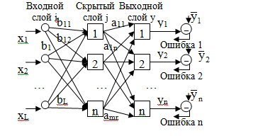
There can be several hidden layers, so the NS is multilayer.

– vector of reference signals (desired)

yi is the vector of real (output) signals

xi is the vector of input signals.

Supervised learning strategy

Typical steps:

1) Select the next training pair from the training set .

x is the input vector;

is the corresponding desired (output vector).

Feed the input vector x to the input of the NN.

2) Calculate the output of the network y - the real output signal.

Previously, the weight coefficients aij and bij are set arbitrarily randomly.

3) Calculate the deviation (error):

4) Correct the weights aij and bij of the network so as to minimize the error.

5) Repeat steps 1-4.

The process is repeated until the error on the entire training set is reduced to the required value.

Forward signal X through the network:

A pair is taken from the training set. For each layer, starting from the first, Y is calculated: Y = F(X A),

where A is the layer weight matrix;

F is the activation function.

Calculations - layer by layer.

Reverse error pass on NS:

The weights of the output layer are adjusted. For this, a modifiable delta rule is applied.

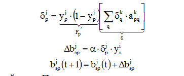
Rice. Training one weight from neuron p in hidden layer j to neuron q in output layer k

For the output neuron, the error signal is first found

εq is multiplied by the derivative of the contraction function calculated for this layer k neuron. We get the value δ:

Δapqk = α δqk ypj,

where α is the learning rate coefficient (0.01≤ α<1) – const, подбирается экспериментально в процесса обучения.

ypj is the output signal of neuron p of layer j.

is the value of the weight in the bundle of neurons p→q at step t (before correction) and step t+1 (after correction).

Adjusting the weights of the hidden layer.

Consider a hidden layer neuron p. When jumping forward, this neuron transmits its output signal to the neurons of the output layer through the weights connecting them. During training, these weights function in reverse order, passing the value of δ from the output back to the hidden layer.

And so for each couple. The process ends if for each X NS will produce

Forecasting with the help of NS. window method.

The time series xt, t=1,2…T is given. The problem of forecasting is reduced to the problem of pattern recognition on the neural network.

The method of identifying patterns in a time series based on NN is called “windowing” (window method).

Two windows Wi (input) and Wo (output) of fixed size n and m, respectively, are used for the observed data set.

These windows are able to move with some step S along the curve (series) along the time axis. The result is a sequence of observations:

The first window, Wi, scans the data, sends it to the input of the National Assembly, and Wo to the output. The pair Wji→Wj0, j=1..n obtained at each step forms a training pair (observation). After training, the NN can be used for prediction.

07.10.2013 Tyler Chessman

Understanding the key ideas of time series forecasting and knowing some of the details will give you an advantage in using the forecasting capabilities in SQL Server Analysis Services (SSAS)

This article will describe the basic concepts necessary for mastering data mining technologies. In addition, we will cover some subtleties so that when you encounter them in practice, you will not be discouraged (see the sidebar "Why data mining is so unpopular").

From time to time, SQL Server professionals need to make forward-looking estimates of future value, such as revenue or sales forecasts. Organizations sometimes use data-mining technology in building predictive models to provide these estimates. Once you understand the basic concepts and some of the details, you will begin to successfully use the forecasting capabilities of SQL Server Analysis Services (SSAS).

Forecasting methods

There are various approaches to forecasting. For example, the Forecasting Methods website (forecastingmethods.org) distinguishes various categories of forecasting methods, including casual (otherwise called economic-mathematical), expert modeling (subjective), time series, artificial intelligence, forecast market, probabilistic forecasting, forecasting modeling, and the method prediction based on reference classes. The Forecasting Principles website (www.forecastingprinciples.com) provides an overview of methods in a methodological tree, primarily separating subjective methods (i.e. methods used when there is insufficient data to quantify) and static methods (i.e. methods used when relevant numerical data available). In this article, I will focus on time series forecasting, a type of static approach in which the accumulated data is sufficient to predict indicators.

Time series forecasting assumes that data obtained in the past helps explain values ​​in the future. It is important to understand that in some cases we are dealing with details that are not reflected in the accumulated data. For example, a new competitor will emerge that could adversely affect future earnings or rapid changes in the composition of the labor force that could affect unemployment rates. In such situations, time series forecasting cannot be the only approach. Often different forecasting approaches are combined to provide the most accurate forecasts.

Understanding the basics of time series forecasting

A time series is a collection of values ​​obtained over a period of time, usually at regular intervals. Common examples include weekly sales, quarterly spending, and monthly unemployment rates. Time series data is presented in a graphical format, with the time interval along the plot's x-axis and values ​​along the y-axis, as shown in Figure 1.

When looking at how a value changes from one period to another, and how to predict values, one should keep in mind that time series data has some important characteristics.

• Base level. The baseline is usually defined as the average of the time series. In some forecasting models, the baseline is usually defined as the starting value of the series data.
• Trend (Trend). A trend generally shows how a time series changes from one period to the next. In the example shown in Figure 1, the number of unemployed tends to increase from the beginning of 2008 until January 2010, after which the trend line goes down. Information on the sample data set used to construct the charts in this article can be found in the sidebar "Calculating the Unemployment Rate."
• Seasonal fluctuations. Some values ​​tend to rise or fall depending on certain periods of time, such as the day of the week or the month of the year. Consider the example of retail sales, which often peak around the Christmas season. In the case of unemployment, we see a seasonal trend with highs in January and July and lows in May and October, as Figure 2 shows.
• Noise. Some prediction models include a fourth characteristic, noise, or error, which refers to random fluctuations and non-uniform movements in the data. Noise will not be considered here.

So by identifying the trend, overlaying the trendline on the baseline, and identifying the seasonal component that might be present in the data analysis, you have a predictive model that can be used to predict values:

Predicted Value = Baseline + Trend + Seasonal

Determination of the base level and trend

The only way to determine the base value and the trend is to use the regression method. The word "regression" here refers to the consideration of the relationship between variables. In this case, there is a relationship between the independent time variable and the dependent variable of the number of unemployed. Note that the independent variable is sometimes called the predictor.

Use a tool like Microsoft Excel to apply the regression method. For example, you can perform an automatic calculation in Excel and add a trendline to a time series plot using the Trendline menu in the Chart Tools Layout tab or the PivotChart Tools Layout tab in the Excel 2010 or Excel 2007 panel. In Figure 1, I added a straight trendline by selecting Mode Linear trendline in the Trendline menu. I then selected More Trendline Options from the Trendline menu, and then the Display Equation on chart and Display R-squared value on chart options, see Figure 3.

Figure 3: Trend Options in Excel

This process of fitting a trend line to the accumulated data is called linear regression. As we can see in Screen 1, the trend line is calculated according to the equation where the base level (8248.8) and the trend (104.67x) are determined:

y = 104.67x + 8248.8

You can think of a trendline as a series of linked x-y coordinates where you can plug in a time span (i.e. x-axis) to get a value (y-axis). Excel determines the "best" trendline using the least squares method (defined as R² in Figure 1). A least squares line is a line that minimizes the squared vertical distance from each point on a trend line to the corresponding point on the line. RMS values ​​allow you to determine that deviations above or below the actual line do not balance each other. In Screen 1, we see that R² = 0.5039, which means that the linear relationship explains 50.39% of the changes in unemployment statistics over time.

Determining an accurate trendline in Excel often involves trial and error, along with visual inspection. In Screen 1, a straight trend line is not the best fit. Excel offers other options for the trend line, which you see in Figure 3. In Figure 4, I added a four-period moving average line, which is based on the arithmetic average of the current and last set periods of the time series.

Also, I added a polynomial trendline by applying an algebraic equation to plot the line. Note that the polynomial trend line has an R² value of 0.9318, which determines the best ratio in expressing the relationship between the independent and dependent variables. However, a higher R² does not necessarily mean that the trendline will provide predictive value. There are other methods for calculating accurate forecasts, which I will briefly describe below. Some trendline options in Excel (for example, linear, polynomial trendlines) allow you to make forecasts forward as well as backward, taking into account the number of periods, plotting the resulting values ​​on a graph. To some, the expression "forecast in the opposite direction" may seem strange. It is best to present this with an example. Let's assume that a new factor - a rapid increase in public sector jobs (eg, jobs in Homeland Defense in the early 2000s, temporary workers of the US Census Bureau) - caused a rapid fall in the unemployment rate. You need to project the rate of growth of the new job sector backwards over several months, and then recalculate the unemployment rate to arrive at a smoothed rate of change.

You can also manually apply the trendline equation to calculate values ​​for the future. In Figure 5, I added a polynomial trendline with a 6-month forecast, first removing the data for the last 6 months (that is, from April to September 2012) from the original time series.

If you compare Screen 5 with Screen 1, you can see that the polynomial forecasts have an uptrend, which is not in line with the downtrend (trend) of the actual time series.

There are two important points to make about regression.

• As mentioned above, linear regression includes one independent and one dependent variable. To understand how additional independent variables might explain changes in the dependent variable, try building a multiple regression model. In the context of predicting the number of unemployed in the United States, you can increase R² (and the accuracy of the forecast) by taking into account the growth rate of the economy, the US population, and the growth in the number of employed workers. SSAS can fit many variables (i.e. regressors) into a time series forecasting model.
• Time series forecasting algorithms, including those used in SSAS, calculate autocorrelation, which is the correlation between adjacent values ​​in a time series. A prediction model that directly includes autocorrelation is called an autoregressive (AR) model. For example, a linear regression model builds a trend equation based on a period (for example, 104.67 * x), while an AR model builds an equation based on previous values ​​(for example, -0.417 * unemployed (-1) + 0.549 * employed (-one)). The AR model potentially increases the accuracy of the forecast, as it takes into account additional information beyond the trend and the seasonal component.

Taking into account the seasonal component

The seasonal component in the structure of the time series usually appears in connection with either the day of the week, or the day of the month, or the month of the year. As noted above, the number of unemployed in the US typically rises and falls in a given calendar year. This is true even when the economy is growing, as shown in Figure 2. In other words, to make an accurate forecast, you must take into account the seasonal component. One common approach is to apply a seasonally adjusted method. In Practical Time Series Forecasting: A Hands-On Guide, Second Edition (CreateSpace Independent Publishing Platform, 2012), author Galit Shmueli recommends using one of three methods:

• moving average calculation;
• time series analysis at a less detailed level (for example, consider changes in the number of unemployed quarterly rather than monthly);
• analysis of individual time series (and calculation of forecasts) by season.

The base level and trend are determined when calculating the forecast, taking into account the smoothed time series. Optionally, a seasonal component or adjustment can be re-applied to the forecast values, taking into account the initial values ​​of the seasonal factor when working with the Holt-Winters method. If you want to see how seasonally factored calculations are made in Excel, type "Winters method in Excel" into an Internet search bar. For an extended explanation of the Holt-Winters method, see Wayne L. Winston Microsoft Office Excel 2007: Data Analysis and Business Modeling, Second Edition (Microsoft Press, 2007).

In many data mining packages, such as SSAS, time series forecasting algorithms automatically account for seasonal fluctuations by measuring seasonal relationships and incorporating them into the forecasting model. However, you may want to install hints about the structure of seasonal changes.

Prediction Model Measurement Accuracy

As already mentioned, the original model (if the least squares method is applied) does not necessarily ensure the accuracy of the forecasts. The best way to check the accuracy of predictive estimates is to divide the time series into two data sets: one for building (i.e. training) the model and the other for validation. The validation dataset will be the most recent part of the input dataset, and it ideally spans a time frame equal to the future forecast timeline. To test (validate) the model, the predicted values ​​are compared with the actual values. Note that once you have validated, the model may be rebuilt using the entire time series, so it is desirable to use the latest actual values ​​to predict future values.

When measuring the accuracy of a predictive model, two questions typically arise: how to determine the accuracy of the predictive estimate, and how much historical data to use to train the model.

How to determine the accuracy of a predictive estimate? In some scenarios, values ​​projected above actual values ​​may not be desirable (for example, in investment forecasts). In other situations, lower-than-actual predicted values ​​can be devastating (for example, predicting the lowest of the auction item's winning prices). But in cases where you want to calculate an estimate for all forecasts (whether the forecast values ​​are higher or lower than the real values), you can start by quantifying the error in a single forecast using the definition:

error = predicted value - actual value

With this definition of error, there are two most popular methods for measuring accuracy: this is the average absolute error, that is, mean absolute error (MAE) and the average absolute percentage error, or mean absolute percentage error (MAPE). In the MAE method, the absolute values ​​of prediction errors are summed and then divided by the total number of predictions. The MAPE method calculates the average absolute deviation from the forecast in percent. To see examples of how to use these and other methods to measure the quality of predictive estimates, an Excel template (with sample predictive data and accuracy factors) can be found on the Demand Metrics Diagnostics Template web page (demandplanning.net/DemandMetricsExcelTemp.htm).

How much historical data should be used to train the model? When working with a time series that has a long history, you may want to include all historical data in the model. However, sometimes the additional history does not improve the accuracy of forecasting. Historical data can even distort the forecast if past conditions differ significantly from those in the present (for example, the composition of the labor force now and in the past is different). I haven't come across any particular formula or practical method that would suggest how much historical data to include, so I suggest starting with time series that are several times larger than the forecast time intervals and then checking for accuracy. Next, try rounding the history number up or down and test again.

Time Series Forecasting in SSAS

Time series forecasting first appeared in SSAS in 2005. To calculate predictive values, the Microsoft Time Series algorithm used a single algorithm called autoregressive tree with cross prediction (ARTXP), or autoregressive tree with cross prediction. ARTXP combines autoregression with decision tree data mining so that the prediction equation can change (meaning split) based on certain criteria. For example, a forecasting model will provide a better fit (and greater forecast accuracy) if you first split by date and then by the value of the independent variable, as shown in Figure 6.

Figure 6: An example of an ARTXP decision tree in SSAS

In SSAS 2008, the Microsoft Time Series algorithm began using an algorithm called autoregressive integrated moving average (ARIMA), in addition to ARTXP, to calculate long-range forecasts. ARIMA is considered the industry standard and can be seen as a combination of autoregressive processes and moving average models. In addition, it analyzes historical forecast errors to improve the model.

By default, the Microsoft Time Series algorithm combines the results of the ARIMA and ARTXP algorithms to achieve optimal predictions. You can disable this feature if you wish. Let's take a look at the SQL Server Books Online (BOL) documentation:

“The algorithm trains two different models of the same data: one model uses the ARTXP algorithm and the other uses the ARIMA algorithm. The algorithm then combines the results of the two models to develop the best prediction covering a variable number of time slices. Since the ARTXP algorithm is more suitable for short-term forecasts, it is desirable to use it at the beginning of a series of forecasts. However, if the time slices needed for forecasting go into the future, the ARIMA algorithm is more meaningful.”

When working with time series forecasting in SSAS, you should always keep the following in mind:

• Although SSAS has a Mining Accuracy Chart tab, it does not work with data mining for time series models. As a result, you should manually measure the accuracy using one of the methods mentioned here (for example, MAE, MAPE) using a tool such as Excel to calculate.
• SSAS Enterprise Edition allows you to split a single time series into many "historical models" so you don't have to manually split the data into datasets for model training and validation to check the accuracy of the forecast. From the end user's point of view, there is only one time series model, but you can compare the actual results with the predicted ones within the model, as Figure 7 shows. data.

Next step

In this article, I introduced you to the basics of time series forecasting. We also considered some details of the basic algorithms so that they do not become an obstacle in the processing of time series. As a next step, I suggest you master time series forecasting tools with SSAS. A project that uses the unemployment data provided in this article can serve as a model. You can then check out the TechNet e-tutorial "Intermediate Data Mining Tutorial (Analysis Services - Data Mining)" at technet.microsoft.com/en-us/library /cc879271.aspx.

Why data mining is so unpopular

In the last decade, business intelligence (BI) technologies such as OLAP have become widely used. At the same time, Microsoft has been pushing another BI technology, data mining, in popular tools like Microsoft SQL Server and Microsoft Excel. However, data mining technology has not yet become a leader. Why? While most people can quickly grasp the core concepts of data mining, the basic details of algorithms are inextricably linked to mathematical concepts and formulas. There is a big "divergence" between a high level of abstract understanding and detailed execution. As a result, data mining is viewed as a "black box" by IT professionals and industrial customers, which is not conducive to widespread adoption of the technology. This article is my attempt to reduce the "divergence" in time series forecasting.

Unemployment Rate Calculation

In the main article, the data for the graphs is based on information about the working population published by U.S. Bureau of Labor Statistics (http://www.bls.gov/). The BLS releases unemployment figures based on a monthly survey conducted by the US Census Bureau (BLS) that extrapolates the total number of employed and unemployed. Specifically, BLS applies the formula:

Unemployment rate = unemployed/(unemployed + employed)

It is noteworthy that when it comes to the unemployment rate, the media usually gives a seasonally adjusted coefficient. Seasonal adjustment is carried out using a common model called the autoregressive integrated moving average (ARIMA). It is essentially the same algorithm used by many data mining packages for time series forecasting, including SQL Server Analysis Services (SSAS). For more information on the ARIMA model used by the BLS, visit the X-12-ARIMA Seasonal Adjustment Program web page (www.census.gov/srd/www/x12a/). Note that in the sample design for this article, I used seasonally and non-seasonally adjusted values.

Mastering Time Series Forecasting

Facebook

Twitter

In contact with

Classmates

Google+