Determination of the present value of cash flows. Future value of money Calculation of simple and compound, nominal and effective interest
When placing capital in investment projects, securities, real estate, commercial banks, etc. It is important to correctly plan the timely return of the invested amount and obtain the expected economic effect. Here comes the theory of the revaluation of money or concept of change in the value of money over time, which is based on the fact that, under the influence of various factors, the value of money changes over time taking into account the rate of profit in the money market, which is the rate of interest. In this case loan interest - This is the amount of income from the use of money in the money market. Considering that the investment process takes a long time, in investment practice it is often necessary to compare the value of money at the beginning of its investment with the value of money when it is returned in the form of future profits, depreciation charges, etc. The principle of the time value of money is based on the fact that A currency unit is worth more today than in the future. A key role in transforming the value of funds over time, that is, comparing the value of funds when they are invested and returned, is played by two basic concepts: the future value of money and its actual (present, current) value.
Future value of money - This is the amount into which the funds invested today (currently) are converted after a certain period of time, taking into account a certain interest rate.
Determining the future value of money is associated with the process of increasing this value. Build-up is a method of constructing the real value of funds into their value in a future period, used to estimate the future value of an investment; This is a gradual increase in the amount of the deposit by adding the amount of interest (interest payments) to its original amount. This amount is calculated using the so-called interest rate. In investment calculations, the interest rate is used not only as a tool for increasing the value of funds, but also in a broad sense - as a measure of the degree of profitability of investment operations.
The discounting method is also associated with the increase, as a method of increasing the amount of funds - this is a method of reducing the future value of funds to their value in the current period (to the real value of money).
Future cash flows can be of the following types:
- Unit cash flow- amount paid in one lump sum;
- Annuity- uniform cash flows that arrive regularly (mortgage payments, insurance premiums, coupon or interest payments on bonds, lease payments, etc.).
There are:
- Ordinary annuity- uniform cash flows carried out at the end of the payment period;
- Series of equal payments (annuity obligation) - payments made at regular intervals at the beginning of a specified period.
Present (current, modern) value of money - This is the sum of future cash receipts, raised taking into account a certain interest rate (the so-called "discount rate, discount factor"), to the present (current) period.
Determining the present value of money is associated with the process of discounting this value; it is an operation inverse to increasing the amount of money at a specified final amount. In this case, the interest amount is calculated from the final amount (future value) of funds. This situation arises in cases where it is necessary to determine how much money needs to be invested today in order to receive a pre-agreed amount after a certain period of time.
Determining the time value of money is necessary to summarize the cash flows that come in over different periods of time. For example, if you have determined the present value of a single receipt and the present value of an annuity, then you can sum these cash flows to determine the total amount of receipts, which is important for determining the income stream from the assets.
When carrying out financial and economic calculations related to investing funds, the processes of increasing and discounting value can be carried out both simple, as well as compound interest. The simple interest technique is used when it is necessary to determine the value of cash flows for short-term financial instruments, that is, when the maturity of the loan is less than a year, and compound interest - when the maturity is more than a year.
The amount of money borrowed (borrowed) or invested (invested) is called capital (initial cost). After a specified period of time, the person using the money (the borrower) must return the capital and capital gains. Capital gains are calculated as a percentage of the principal amount. This value is called the interest rate, and the method of calculating profit is the simple interest (interest) method.
Simple interest - this is a method of accrual from the current value of the deposit at the end of one payment period, determined by the investment conditions (month, quarter, etc.); This is a method of calculating the income the lender receives from the borrower for the money lent. They are accrued on the same amount of borrowed capital throughout the entire loan repayment period.
The basic concepts of financial and economic calculations are:
A)percent - this is income from the provision of capital in debt in various forms (loans, credits, etc.) or from investments of an industrial or financial nature;
b)interest rate - a value characterizing the intensity of interest accrual;
V)increased primary (invested) amount - this is an increase in this amount due to accrued interest; the ratio of the accumulated amount in the primary is called the accumulation multiplier; the growth factor shows how many times the primary capital has grown;
G)accrual period is the time interval for which interest is calculated.
Simple interest is determined by the formula:
When using simple interest, when the agreement term does not correspond to a whole number of years, the interest accrual period is expressed as a fraction, that is, as the ratio of the number of months (days) of the agreement to the number of months (days) in the year:

Compound interest techniques are used to determine the value of cash flows generated by long-term financial instruments.
Compound interest - this is the amount of profit that is generated as a result of investment, provided that the amount of accrued interest (simple) is not paid after each period, but is added to the amount of the main deposit and in the next payment period itself generates income.
This method of calculating profits in a future period is called compounding, or calculating future value. Each step of this process is called compound(accrual), and the result of accrual - compound interest.
There are two methods of calculating compound interest: where-italic and anti-compound.
Decursive (next) way provides for the accrual of interest at the end of each accrual time interval. The amount of interest is determined based on the amount of capital used.
Antisipative (preliminary) method provides for the accrual of interest at the beginning of each time interval. In world practice, the decursive method of calculating interest has become widespread. The anticipatory method of calculating interest is not used so often, only during periods of high inflation. According to the decursive method of calculating interest, the accumulated amount of debt (payment) is determined by the formula.
Net present value is the sum of the current values of all predicted cash flows, taking into account the discount rate.
The net present value (NPV) method is as follows.
1. The current cost of costs (Io) is determined, i.e. The question of how much investment needs to be reserved for the project is decided.
2. The current value of future cash receipts from the project is calculated, for which the income for each year CF (cash flow) is reduced to the current date.
The calculation results show how much money would need to be invested now to receive the planned income if the income rate were equal to the barrier rate (for an investor, the interest rate in a bank, in a mutual fund, etc., for an enterprise, the price of total capital or through risks). Summing up the current value of income for all years, we obtain the total current value of income from the project (PV):
3. The present value of investment costs (Io) is compared with the present value of income (PV). The difference between them is the net present value of income (NPV):
NPV shows the investor's net gains or net losses from investing money in a project compared to keeping the money in a bank. If NPV > 0, then we can assume that the investment will increase the wealth of the enterprise and the investment should be made. At NPV
Net present value (NPV) is one of the main indicators used in investment analysis, but it has several disadvantages and cannot be the only means of evaluating an investment. NPV measures the absolute value of the return on an investment, and it is likely that the larger the investment, the greater the net present value. Hence, it is not possible to compare multiple investments of different sizes using this indicator. In addition, NPV does not determine the period over which the investment will pay off.
If capital investments associated with the upcoming implementation of the project are carried out in several stages (intervals), then the NPV indicator is calculated using the following formula:
![]() , Where
, Where
CFt - cash inflow in period t;
r - barrier rate (discount rate);
n is the total number of periods (intervals, steps) t = 1, 2, ..., n (or the duration of the investment).
Typically for CFt the t value ranges from 1 to n; in the case where CФо > 0 is considered a costly investment (example: funds allocated for an environmental program).
Defined by: as the sum of the current values of all predicted, taking into account the barrier rate (discount rate), cash flows.
Characterizes: investment efficiency in absolute values, in current value.
Synonyms: net present effect, net present value, Net Present Value.
Acronym: NPV
Flaws: does not take into account the size of the investment, the level of reinvestment is not taken into account.
Eligibility Criteria: NPV >= 0 (the more the better)
Comparison conditions: To correctly compare two investments, they must have the same investment costs.
Example No. 1. Calculation of net present value.
The investment amount is $115,000.
Investment income in the first year: $32,000;
in the second year: $41,000;
in the third year: $43,750;
in the fourth year: $38,250.
The size of the barrier rate is 9.2%
Let's recalculate cash flows in the form of current values:
PV 1 = 32000 / (1 + 0.092) = $29304.03
PV 2 = 41000 / (1 + 0.092) 2 = $34382.59
PV 3 = 43750 / (1 + 0.092) 3 = $33597.75
PV 4 = 38250 / (1 + 0.092) 4 = $26899.29
NPV = (29304.03 + 34382.59 + 33597.75 + 26899.29) - 115000 = $9183.66
Answer: The net present value is $9,183.66.
The formula for calculating the NPV (net present value) indicator taking into account the variable barrier rate:

NPV - net present value;
CFt - inflow (or outflow) of funds in period t;
It is the amount of investments (costs) in the t-th period;
ri - barrier rate (discount rate), fractions of a unit (in practical calculations, instead of (1+r) t, (1+r 0)*(1+r 1)*...*(1+r t) is used, because . the barrier rate can vary greatly due to inflation and other components);
N is the total number of periods (intervals, steps) t = 1, 2, ..., n (usually the zero period implies the costs incurred to implement the investment and the number of periods does not increase).
Example No. 2. NPV with a variable barrier rate.
Investment size - $12800.
in the second year: $5185;
in the third year: $6270.
10.7% in the second year;
9.5% in the third year.
Determine the net present value for the investment project.
n =3.
Let's recalculate cash flows in the form of current values:
PV 1 = 7360 / (1 + 0.114) = $6066.82
PV 2 = 5185 / (1 + 0.114)/(1 + 0.107) = $4204.52
PV 3 = 6270 / (1 + 0.114)/(1 + 0.107)/(1 + 0.095) = $4643.23
NPV = (6066.82 + 4204.52 + 4643.23) - 12800 = $2654.57
Answer: The net present value is $2,654.57.
The rule according to which, from two projects with the same costs, the project with a large NPV is selected does not always apply. A project with a lower NPV but a short payback period may be more profitable than a project with a higher NPV.
Example No. 3. Comparison of two projects.
The cost of investment for both projects is 100 rubles.
The first project generates a profit equal to 130 rubles at the end of 1 year, and the second 140 rubles after 5 years.
For simplicity of calculations, we assume that barrier rates are equal to zero.
NPV 1 = 130 - 100 = 30 rub.
NPV 2 = 140 - 100 = 40 rub.
But at the same time, the annual profitability calculated using the IRR model will be equal to 30% for the first project, and 6.970% for the second. It is clear that the first investment project will be accepted, despite the lower NPV.
To more accurately determine the net present value of cash flows, the modified net present value (MNPV) indicator is used.
Example No. 4. Sensitivity analysis.
The investment amount is $12,800.
First year investment income: $7,360;
in the second year: $5185;
in the third year: $6270.
The size of the barrier rate is 11.4% in the first year;
10.7% in the second year;
9.5% in the third year.
Calculate how the net present value would be affected by a 30% increase in investment income?
The initial value of the net present value was calculated in example No. 2 and is equal to NPV ex = 2654.57.
Let's recalculate cash flows in the form of current values, taking into account sensitivity analysis data:
PV 1 ah = (1 + 0.3) * 7360 / (1 + 0.114) = 1.3 * 6066.82 = $7886.866
PV 2 ah = (1 + 0.3) * 5185 / (1 + 0.114)/(1 + 0.107) = 1.3 * 4204.52 = $5465.876
PV 3 ah = (1 + 0.3) * 6270 / (1 + 0.114)/(1 + 0.107)/(1 + 0.095) = 1.3 * 4643.23 = $6036.199
Let's determine the change in net present value: (NPV ach - NPV out) / NPV out * 100% =
= (6036,199 - 2654,57) / 2654,57 * 100% = 127,39%.
Answer. A 30% increase in investment income resulted in a 127.39% increase in net present value.
Note. Discounting cash flows with a time-varying barrier rate (discount rate) corresponds to “Methodological guidelines No. VK 477...” clause 6.11 (p. 140).
Net present value
Copyright © 2003-2011 by Altair Software Company. Potential programs and projects.
Simple and compound interest.. 2
Problems and solutions. 7
Frequency of compounding interest. 9
Current value of money. 10
Annuity. 14
Loan amortization. 17
The impact of inflation. 18
SECURITIES.. 20
Bond price. 21
Bond yield. 30
Bond yield. 30
Price and yield of certificates of deposit and bills of exchange. 38
Stock price and return. 40
Preferred shares. 41
Ordinary shares. 42
Stock return. 49
Risk analysis. 52
Risk of investing in securities. 53
Risk and its types.. 53
Risk measurement. 54
Return and risk of a securities portfolio. 67
Reducing risk through diversification. 67
Portfolio analysis. 68
Relationship between covariance and standard deviation of a portfolio. 71
Optimization of a portfolio consisting of two securities. 74
Portfolio optimization according to Markowitz. 77
CAPITAL ASSET VALUATION MODEL... 81
Options.. 87
The essence of an option, basic concepts. 87
Option price, Black-Scholes model. 92
Accounting for the time value of money
Simple and compound interest
The decision to invest capital is determined in most cases by the amount of income that the investor expects to receive in the future. When making such decisions, the time factor plays a very important, if not decisive, role. In this regard, the problem arises of accounting for expenses and income spread over time. To solve it, you need a correct understanding of the time value of money and the method of discounting cash flows.
The concept of time value of money can be formulated as follows: money today is worth more than the same amount we will receive in the future. This fact is due to the following circumstances.
1. Today's money can be invested and receive additional money in the form of interest.
2. The purchasing power of money may fall over time due to inflation.
3. You cannot be completely sure that you will receive money in the future.
Thus, to make time-effective financial decisions, it is necessary to use appropriate methods that take into account the time aspect of the value of money.
Transformations of cash flow elements are carried out by applying accumulation and discounting operations. Accumulation is the process of determining the future value of money. Discounting is the process of bringing money to its current value. In the first case, they move from the “present” to the future, in the second, on the contrary, from the future to the present. In both cases, using the compound interest scheme, it is possible to obtain an assessment of cash flow from the perspective of the future or “present”.
The future value of money FV (future value) represents the future value of the amount of funds that the investor currently has, based on the expected rate of return, the accumulation period and the frequency of interest. Estimation of the future value of money is associated with the process of accumulation, which is a gradual increase in the original value by adding income to it, calculated taking into account the rate of return.
The given formulas are among the basic ones in financial calculations, therefore, for ease of use, the values of the multipliers FM1(i, n)= (1+i)n and FM2(i, n)=1/ (1+i)n tabulated for different values i And n(This and other financial tables mentioned in this section can be found in the literature on financial management and analysis).
Factor PM1(i,p) is called a multiplying factor for a single payment, and its economic meaning is as follows: it shows what the cost of one monetary unit (one ruble, one dollar, etc.) will be equal to through n periods at a given interest rate i. We emphasize that when using financial tables, it is necessary to ensure that the length of the period and the interest rate correspond. So, if the base period for calculating interest is a quarter, then the quarterly rate should be used in the calculations.
Factor PM2(i,p) is called the discount factor for a single payment, and its economic meaning is as follows: it shows the “today’s” price of one monetary unit of the future, i.e., what is the value of one monetary unit (for example, one ruble) that will be received from the current point of view or paid via n periods from the moment of calculation, at a given interest rate (yield) i. The term “present value” should not be taken literally, since discounting can be performed at any point in time, not necessarily the current moment.
The most important parameter that determines the present and future value of money is the interest rate. The interest rate is the ratio of the amount of income for a fixed period of time to the amount of debt. The time interval to which the interest rate is assigned is called the accrual period. Most often in practice, annual rates are used. However, the accrual period can be half a year, a quarter, a month, or even a day. Interest can be paid as it accrues or added to the principal amount. In the latter case, we talk about interest capitalization. The process of increasing the amount of money over time due to the addition of interest is called accumulation.
The interest rate on any type of loan or fixed income instrument depends on a number of factors, the most important of which are the unit of account, the payment term and the risk of the borrower defaulting on the terms of the loan agreement.
The absolute amount of income from lending money is called interest. In this case, the percentage is an absolute value expressed in monetary units, and not a hundredth part of a number.
If we denote by I – interest, i – interest rate and P – amount of debt, then the relationship between the values is determined by the following ratio:
i = I / P.
Simple and compound interest
Simple interest is the interest at which its value is calculated on the initially invested amount of funds. In this case, the amount of interest accrued in previous periods is not taken into account in the process of subsequent accrual.
In the case of compound interest, interest is calculated on a constantly increasing basis, taking into account interest accrued in previous periods. It is used in cases where interest on loans (deposits) is not paid immediately, but is added to the amount of the principal debt. This procedure is called capitalization.
The quantities (1+n*i) and (1+i)n are called coefficients (multipliers) for increasing simple and compound interest, respectively.
Example. Let's assume that you deposited 1000 rubles into your bank account. (PV) The interest rate is 10% per annum. It is necessary to calculate the amount that you will receive in 5 years, provided that you do not withdraw interest.
Let's calculate the future value step by step. At the end of the first year you will have an amount in your account equal to
FV1= 1000* (1+0.1) = 1100 rub.
The amount received consists of 1000 rubles, with which this financial transaction began, plus interest in the amount of 100 rubles. Future value 1000 rub. by the end of the first year it amounted to 1100 rubles.
If you leave 1100 rub. for another year, then at the end of the second year you will have the amount
FV2= 1100* (1+0.1) = 1210 rub.
This amount can be represented in the form of three components. Initial money - 1000 rubles, interest for the first year - 100 rubles. and for the second year - 100 rubles. Interest accrued on the principal amount of the deposit is called simple interest. The third component is equal to 10 rubles. and represents the interest received in the second year, which was accrued on the 100 rubles received as interest in the first year. Interest calculated on previously accrued interest is called compound interest. The total amount of interest charges is 210 rubles. consists of simple interest (200 rubles) and compound interest (10 rubles).
Continuing the presented chain of calculations, we can calculate the amount in the account after 5 years.
FV5= 1000* (1+0.1)5 = 1610.51 rub.
Thus, the future value is 1000 rubles. after five years at a loan interest rate of 10% per annum it is 1610.51 rubles. The total amount of interest accrued for five years is 610.51 rubles, of which 500 rubles. are simple interest and 110.51 are compound interest.
Example. You are 20 years old and you decide to deposit 1000 rubles into your account. for a period of 40 years at a rate of 10% per annum. How much money will be in your account when you are 60 and retire. How much of this amount will be simple and compound interest?
FV = 1000 * (1+0.1)40 = 45259.26
The received amount consists of the initial amount equal to 1000 rubles, simple interest 1000 * 0.1 * 40 = 4000 rubles. and compound interest equal to 40259.26 rubles.
Consider the effect of increasing the interest rate to 11%.
FV = 1000 * (1+0.11)40 = 65000.87 rub.
In this example, a seemingly insignificant increase in the interest rate by 1% resulted in an additional amount of RUB 24,741.61.
Along with the problems of compound interest compounding, in the practice of financial calculations there are tasks that require simple interest compounding. In this case, interest is accrued only on the principal amount of the deposit. These include the problem of determining the price of short-term financial instruments, as well as long-term instruments if interest is not added to the principal debt, but is paid. The formula for determining the future value of money for this case will be:
FV = PV * (1+n*i).
In this formula we used previously accepted notation.
Example. Let's return to the example discussed above. You are 20 years old and you decide to deposit 1000 rubles into your account. for a period of 40 years at a rate of 10% per annum. How much money will be in your account when you are 60 and retire.
FV = 1000 * (1+40*0.1) = 1000+4000 = 5000
The amount received is the sum of the initial amount equal to 1000 rubles. and simple interest 1000*0.1*40 = 4000 rubles.
Interest can be determined not only by calculations from the present to the future, but also from the future to the present. In this case, the percentage represents a discount from some final amount. For example, in the banking practice of discounting bills of exchange, the cost of a bill of exchange is the final amount from which a discount is made at a certain rate, called the discount rate. The difference between the cost of a bill and the amount that the bank issues on this bill is called a discount.
Problems and solutions
1. 10,000 rubles are deposited on a deposit for a period of two years. What amount should the investor receive at the end of the term when calculating simple (compound) interest at a rate of 18% per annum?
For the case of simple interest we get:
FV = PV *(1+n*i) = 10000*(1+2*0.18) = 13600 rub.
For the case of compound interest:
FV = PV *(1+ i)n= 10000*(1+*0.18)2= 13924 rub.
2. Find the period of time during which the initial deposit amount will double for the case of simple and compound interest rates equal to 10%.
For the case of a simple bet
FV = 2*PV = PV *(1+n*i),
n = (2-1)/0.1 =10 years.
For a complex bet
FV = 2*PV = PV *(1+i)n
n*Ln(1+0,1) =Ln2,
n= Ln2/ Ln(1+0.1) = 0.69/0.095 = 7.26 years.
3. Find the interest rate (simple and complex) at which the initial deposit amount will double in ten years.
For the case of a simple bet
FV = PV *(1+n*i),
FV = 2*PV = PV *(1+10*i),
For a complex bet
FV = 2*PV = PV *(1+i)10
i = 2 1/10 – 1 = 0.072.
4. On your bank deposit, interest is calculated based on a “floating” rate, which changes every year. Three years ago you deposited 10,000 rubles into your account when the interest rate was 15%. Last year it fell to 12%, and this year it is set at 10%. How much money will you have in your account by the end of this year? Calculations are made for the case of simple and complex bets.
For the case of a simple bet
FV = PV *(1+n1*i1 + n2*i2 + n3*i3) = 10000*(1+1*0.15+1*0.12+1*0.1) = 13700 rub.
For complex bets
FV = PV *(1+ i1)n1 *(1+ i2)n2 *(1+ i3)n3 = 10000* *(1+ 0.15)1*(1+ 0.12)1*(1+ 0 ,1)1 = 10000* 1.15*1.12*1.1 = 14168 rub.
5. RUB 1,000 is deposited in the bank’s urgent savings account. for two years at a rate of 9% per annum, with further extension for the next three years at a rate of 6%. Find the accumulated amount after five years at simple and complex rates.
For the case of a simple bet
FV = PV *(1+n1*i1 + n2*i2) = 1000*(1+2*0.09+3*0.06) = 1360 rub.
For complex bets
FV = PV *(1+ i1)n1 *(1+ i2)n2 = 1000* *(1+ 0.09)2*(1+ 0.06)3 = 1417 rub.
1. Bill worth 100 million rubles. taken into account by the bank 2 years before maturity at a compound rate of 20% per annum. What amount will the holder of the bill receive upon expiration of the contract?
Compounding frequency
The interest rate is usually set as the nominal annual interest rate - this is the initial rate that the bank sets for calculating interest. This rate can also be used to compound interest once a year. In this case, if interest is accrued more often than once a year, for example, quarterly or monthly, the effective annual rate is calculated, which is equivalent to the interest rate if interest is accrued once a year.
Let's assume that the annual interest rate is, for example, 6% per year, with interest compounded monthly. This means that interest is added to your account every month in the amount of 1/12 of 6%, or 0.5%. The effective interest rate can be found from the expressions
FV = (1.005)12 = 1.061678
Ie = 1.06168-1 = 0.061678 = 6.1678% per year.
The general formula for calculating the effective annual interest rate is as follows:
Iе = (1+i/m)m – 1,
I is the nominal annual rate, m is the number of interest accruals per year.
As the compounding frequency increases, the effective interest rate increases. If interest accrues continuously, then the effective interest rate is determined from the ratio
Iе = Lim (1+i/m)m – 1 = ei - 1= 2.71828i -1
m à infinity.
In our example, e 0= 6.1836 per year.
Example. The nominal annual rate is 12% per year. Interest is calculated quarterly. Find the annual effective rate
Ie = (1+0.12/4)4 – 1 = 12.55%.
Current value of money
The procedure for calculating the current (present) value of money is the opposite of calculating the future value. With its help, we can determine how much money needs to be invested today in order to receive a certain amount in the future.
General formula for calculating the present value of 1 rub. after n periods it looks like:
where PV is the current value of money,
FV – future value of money,
n – number of time intervals,
i – discount rate.
Example. What amount must be deposited into the account in order to receive 1000 rubles in five years? (i=10%)
PV = 1000 / (1+0.1)^5 = 620.92 rub.
Thus, to calculate the current value of money, we must divide its known future value by the value (1+i)n. The present value is inversely related to the discount rate. For example, the present value of a monetary unit received in 1 year at an 8% interest rate is
PV = 1/(1+0.08)1 = 0.93,
And at a rate of 10%
PV = 1/(1+0.1)1 = 0.91.
The current value of money is also inversely related to the number of time periods before it is received.
The considered procedure for discounting cash flows can be used when making investment decisions. The most common decision rule is the net present value (NPV) rule. Its essence is that participation in an investment project is advisable if the present value of future cash receipts from its implementation exceeds the initial investment.
Example. It is possible to buy a savings bond with a nominal value of 1000 rubles. and a repayment period of 5 years for 750 rubles. Another alternative investment option is to place your money in a bank account with an interest rate of 8% per annum. It is necessary to evaluate the feasibility of investing in the purchase of a bond.
To calculate NPV as an interest rate, or more generally as a rate of return, it is necessary to use the opportunity cost of capital. The opportunity cost of capital is the rate of return that can be obtained from other investment avenues. In our example, an alternative type of investment is to place money on a deposit with a yield of 8%.
A savings bond provides cash receipts of RUB 1,000. in 5 years. The present value of this money is
PV = 1000/1.08^5 = 680.58 rub.
Thus, the current value of the bond is 680.58 rubles, while they offer to buy it for 750 rubles. The net present value of the investment will be 680.58-750=-69.42, and investing in the purchase of a bond is not advisable.
The economic meaning of the NPV indicator is that it determines the change in the financial condition of the investor as a result of the implementation of the project. In this example, if the bond is purchased, the investor’s wealth will decrease by 69.42 rubles.
The NPV indicator can also be used to evaluate various options for borrowing funds. For example, you need to borrow $5,000. to purchase a car. The bank offers you a loan at 12% per annum. Your friend can borrow $5,000 if you give him $9,000. in 4 years. It is necessary to determine the optimal borrowing option. Let's calculate the current value of $9,000.
PV = 9000/(1+0.12)^4 = $5719.66
Thus, the NPV of this project is 66 = -719.66 dollars. In this case, the best borrowing option is a bank loan.
To calculate the effectiveness of investment projects, you can also use the internal rate of return (IRR). The internal rate of return is the value of the discount rate that equalizes the present value of future revenues and the present value of costs. In other words, IRR is equal to the interest rate at which NPV = 0.
In the above example of purchasing a bond, the IRR is calculated from the following equation
750 = 1000/(1+IRR)^5
Cash flow assessment
Most financial decisions involve dealing with multiple cash flows, that is, cash payments or receipts occurring over a number of time intervals. As an example, we can consider the purchase of a bond on which periodic interest payments are expected, the formation of the funded part of the pension through periodic contributions by the employer and employee.
Flow Elements WITH can be either independent or interconnected by a certain algorithm. Time periods are most often assumed to be equal. It is also considered that receipts generated within one time period occur either at its beginning or at its end, that is, they are not distributed within the period, but are concentrated at one of its boundaries. In most cases, cash receipts are considered tied to the end of the time interval.
Cash flow assessment can be performed as part of solving two problems: (a) direct, i.e., an assessment is carried out from the perspective of the future (an accumulation scheme is implemented); (b) reverse, i.e., an assessment is carried out from the perspective of the present (a discounting scheme is implemented).
The direct task involves a total assessment of the increased cash flow, i.e. it is based on future value. In particular, if the cash flow represents regular accruals of interest on invested capital (P) according to the compound interest scheme, then the following formula is the basis for the total assessment of the accumulated cash flow.
FV = Ck * (1+i)k
Example. Every year you deposit 1000 rubles. to an account that pays 10% per annum starting from the date of deposit. How much money will you have in your account after two years if you do not withdraw interest? By the end of the first year, the initial amount is 1000 rubles. will increase to the value
FV1 = 1000* (1+0.1)1 = 1100 rub.
At the beginning of the second year, another 1000 rubles will be added to this amount. and there will be 2100 rubles in the account. By the end of the second year this amount will increase to
FV2 = 2100* (1+0.1)1 = 2310 rub.
Reverse the task involves a summary assessment of discounted (reduced) cash flow. Since individual elements of cash flow are generated at different time intervals, and money has a time value, their direct summation is impossible. Bringing elements of cash flow to one point in time is carried out using the following formula
PV = Ck / (1+i)k
As an example of a problem of this type, we can consider determining the current value of a bond that will be repaid in two years with a par value of 1000 rubles. and a coupon rate of 10%. This bond assumes coupon payments of 100 rubles. at the end of the first and second year. In addition, at the end of the second year the face value of the bond is paid. Taking this into account, the present value of the cash flow will be equal to
PV = 100 / (1+0.1)1 + 100 / (1+0.1)2. + 1000 / (1+0.1)2 = 8438.01 rub.
Annuity
One of the key concepts in financial calculations is the concept of annuity. The logic behind the annuity payment scheme is widely used in the valuation of debt and equity securities, in the analysis of investment projects, as well as in lease analysis.
An annuity is a special case of cash flow. There are two known approaches to its definition. According to the first approach, an annuity is a unidirectional cash flow, the elements of which take place at equal time intervals. The second approach imposes an additional restriction, namely: the elements of cash flow are equal in size. In the further presentation of the material, we will adhere to the second approach. If the number of equal time intervals is limited, the annuity is called a fixed-term annuity. In this case:
C1= NW= ... = Sp= A.
To estimate the future and present value of an annuity, you can use the above formulas, however, due to the specifics of annuities in relation to the equality of cash receipts, they can be significantly simplified.
The formula for calculating the current value of an annuity is
PVA = A/(1+i)+A/(1+i)2 A/(1+i)3+…+A/(1+i)n.
Let us introduce the following notation
As a result we get
PVA=B*(1+C+C2+C3+… +Cn-1) *
Multiplying the left and right sides of the equation by the value C
PVA*C = B*(C+C2+C3+… +Cn) **
Subtracting the equation ** from * we get
PVA*(1-C) = B*(1-Cn).
PVA* = A/(1+i)*.
Multiplying both sides of the equation by (1+i) gives
PVA*i = A*
PVA = A*.
An expression for calculating the future value of an annuity can be derived in a similar way.
FVA = A+A*(1+i)2 A*(1+i)3+…+A*(1+i)n-1.
Let us introduce the notation B=A*(1+i)/ and get
FVA = A*(1+B +B2 B3+…+Bn-1).
Let's multiply both sides of the equation by the value B.
FVA*B = A*(B +B2 B3+…+Bn).
Subtracting this equation from the previous one we get,
FVA*(1-B) = A*(1-Bn).
FVA = A/i*[(1+i)n-1].
Similar to functions FM1(i, n)= (1+i)n and FM2(i, n)=1/ (1+i)n functions FM3(i, n)= 1/i*[(1+i)n-1] FM4(i, n)= and tabulated for different meanings i And p. Economic sense FMZ(i,p), called the multiplying factor for an annuity, is as follows: it shows what the total value of a fixed-term annuity of one monetary unit (for example, one ruble) will be equal to by the end of its validity period. It is assumed that only the accrual of cash amounts is made, and their withdrawal can be made at the end of the annuity period. Factor FM4(i,p) shows the current value of an annuity of one monetary unit for given values of i and n.
Some investment calculations use a perpetual annuity valuation technique. An annuity is called perpetual if cash receipts continue for a sufficiently long time (in Western practice, annuities designed for 50 years or more are classified as perpetual).
In this case, the direct task makes no sense. As for the inverse problem, its solution can be obtained based on the formula
PVA = A*
as n tends to infinity.
The given formula is used to assess the feasibility of purchasing a perpetual annuity. In this case, the amount of annual income is known; as a discount factor i Usually a guaranteed interest rate is accepted (for example, the interest offered by a state-owned bank).
Loan amortization
Many loans, such as home loans and car loans, are repaid in even, periodic payments. Each of them consists of two parts: interest on the balance of the debt and part of its principal amount. After each payment, the remaining debt amount is reduced by the amount already paid. Consequently, in the next payments, the part that contains accrued interest is less than the interest for the previous period, and the part attributable to the payment of the principal amount of the loan is greater than in the previous period.
Let's say you take out a $100,000 loan to buy a house at 9% per annum, with the entire amount plus interest paid back in three annual payments. First we calculate the annual payment, for which we find A, PVA which is $100,000, subject to payment of 9% per annum for three years:
PVA = A*.
A = PVA/.
A = 100000/.
Thus, the annual payment is $39,505.48. Next, you need to determine how much of the $39,505.48 in the first year will be interest and how much will be the principal payment? Since the interest rate is 9% per annum, the interest portion of the first year must be 0.09 x or $9,000. The balance of $39,504.48, or $30,505.48 is the payment amount of the principal amount of $100,000 Thus, after the first payment, the loan balance is $100,000.48, or $52. The process of gradually repaying the loan over its entire life is called loan amortization.
Next, we will calculate payments in the second year. Interest payments in the second year will be $0.09 x $52, or $6,254.51. The balance of $39,504.48 after interest calculation will be $33,250.97—this is the principal payment. The balance after the second payment is therefore $69,494.52.97, or $36,243.54.
The third and final payment covers both interest and the principal amount of $36,243.54 (i.e., 1.09 x $36,243.55 = $39,504.47). The considered repayment schedule for a three-year loan is presented in the table.
|
Initial debt |
Total payment |
Interest paid |
Principal amount paid |
Remaining debt |
|
|
Total |
Analysis of the data presented shows that with each subsequent payment of $39,504.48, the portion attributable to interest decreases, and the portion of the principal amount intended to pay off the principal amount of the loan increases.
Impact of inflation
Inflation has a significant impact on financial decision making. Let's look at saving for old age as an example. At the age of 20, you saved $100 and invested it at the rate of 8% per annum. Calculations show that your $100 investment will grow to $3,192 by the time you turn 65. It must be taken into account that the real purchasing power of money will decrease significantly over 45 years. The things you buy today will cost much more by then. For example, if the prices of all the goods and services you want to buy rise by 8% per year for the next 45 years, your $3,192 will buy you no more than $100 today.
NPV (abbreviation in English - Net Present Value), in Russian this indicator has several variations of the name, among them:
- net present value (abbreviated NPV) is the most common name and abbreviation, even the formula in Excel is called exactly that;
- net present value (abbreviated NPV) - the name is due to the fact that cash flows are discounted and only then summed up;
- net present value (abbreviated NPV) - the name is due to the fact that all income and losses from activities due to discounting are, as it were, reduced to the current value of money (after all, from the point of view of economics, if we earn 1,000 rubles and then actually receive less than if we received the same amount, but now).
NPV is an indicator of the profit that participants in an investment project will receive. Mathematically, this indicator is found by discounting the values of net cash flow (regardless of whether it is negative or positive).
Net present value can be found for any period of time of the project since its beginning (for 5 years, for 7 years, for 10 years, and so on) depending on the need for calculation.
What is it for?
NPV is one of the indicators of project efficiency, along with IRR, simple and discounted payback period. It is needed to:
- understand what kind of income the project will bring, whether it will pay off in principle or is it unprofitable, when it will be able to pay off and how much money it will bring at a particular point in time;
- to compare investment projects (if there are a number of projects, but there is not enough money for everyone, then projects with the greatest opportunity to earn money, i.e. the highest NPV, are taken).
Calculation formula
To calculate the indicator, the following formula is used:
- CF - the amount of net cash flow over a period of time (month, quarter, year, etc.);
- t is the period of time for which the net cash flow is taken;
- N is the number of periods for which the investment project is calculated;
- i is the discount rate taken into account in this project.
Calculation example
To consider an example of calculating the NPV indicator, let's take a simplified project for the construction of a small office building. According to the investment project, the following cash flows are planned (thousand rubles):
| Article | 1 year | 2 year | 3 year | 4 year | 5 year |
| Investments in the project | 100 000 | ||||
| Operating income | 35 000 | 37 000 | 38 000 | 40 000 | |
| Operating expenses | 4 000 | 4 500 | 5 000 | 5 500 | |
| Net Cash Flow | - 100 000 | 31 000 | 32 500 | 33 000 | 34 500 |
The project discount rate is 10%.
Substituting into the formula the values of net cash flow for each period (where negative cash flow is obtained, we put it with a minus sign) and adjusting them taking into account the discount rate, we get the following result:
NPV = - 100,000 / 1.1 + 31,000 / 1.1 2 + 32,500 / 1.1 3 + 33,000 / 1.1 4 + 34,500 / 1.1 5 = 3,089.70
To illustrate how NPV is calculated in Excel, let's look at the previous example by entering it into tables. The calculation can be done in two ways
- Excel has an NPV formula that calculates the net present value, to do this you need to specify the discount rate (without the percent sign) and highlight the range of the net cash flow. The formula looks like this: = NPV (percent; range of net cash flow).
- You can create an additional table yourself where you can discount the cash flow and sum it up.
Below in the figure we have shown both calculations (the first shows the formulas, the second the calculation results):


As you can see, both calculation methods lead to the same result, which means that depending on what you are more comfortable using, you can use any of the presented calculation options.
08.03.2015 21:16 3473
FUNDAMENTALS OF THE THEORY OF MONEY VALUE IN TIME
Measuring the value of real estate in monetary form and the fact that its value is determined, as a rule, by the current value of future income from the ownership and use of real estate requires turning to the theory of the time value of money, which explains the processes of determining the future value of money (accumulation) and bringing money flows to their current value (discounting).
Given that these processes are based on the effect of compound interest, the focus of this chapter will be on the application of standard compound interest functions in valuation procedures and an explanation of their economic content. Specifically, six basic functions will be considered: the accumulated amount (future value) of the unit, the accumulation of the unit over the period, the contribution to the replacement fund, the present value of the unit (reversion), the present value of an ordinary annuity, and the contribution to depreciation of the unit.
Accumulation and discounting processes
As already noted, the value of real estate is expressed in monetary terms. In other words, money is the commodity for which rights regarding real estate are exchanged. But, like any other product, money must have value, i.e. on the corresponding market, the capital market, you can take money for use for a certain period for a certain fee. In the same market, you can give your money for use for a while, expecting to receive a reward for this.
This is clearly illustrated by banking operations. When placing money on bank deposits, in essence, they are transferred for use, and the interest rate that the bank offers on the invested capital is a payment for this use. And, conversely, money borrowed must be returned to the bank in full, along with a certain percentage, as a fee for using this money.
In any case, the amount of money today, which is called the present value, and the amount of money tomorrow, which is called the future value, will differ by the amount of interest income:
where FV is the amount that reflects the future value;
PV - the amount reflecting the current value;
i - interest rate.
Reasoning in a similar way, we can solve the inverse problem of how much PV must be invested today in order to receive a certain amount of FV in the future for a given level of remuneration i:

This problem is called the discounting problem, that is, reducing the future value to the current value, and the coefficient DF=1/(1+i), which is used in this case, is called the discount factor.
Accumulation and discounting operations

Thus, the most important operations that provide the opportunity to compare money at different times are the operations of accumulation and discounting.
Accumulation is the operation of bringing current value into the future.
Discounting is the reduction of future value to current value.
Financial analysis is based on these two operations. One of its main criteria is the interest rate, or the ratio of net income to invested capital. When performing an accumulation operation, it is called the rate of return on capital; when discounting, it is called the discount rate.
Investing in real estate is very similar to using money. Investing money in the purchase and/or construction of real estate involves generating income in the future, not today. Such a renunciation of the current use of money also requires its payment - receiving income on the invested capital. Thus, the future value of any property will be greater than the current value by the amount of this income.
EXAMPLE
A project to invest in the construction of an office building is being considered. The forecast calculation showed that in a year the building could be sold for $400 thousand. It is necessary to determine how much it is worth investing in construction today if the level of income acceptable to the investor is 15%.
Naturally, the rate of return on capital that an investor can accept will be determined by the risk of obtaining that amount of return. The higher the risk of achieving a given amount of income, the higher the rate of payment for capital invested in construction should be.
The above reasoning shows that the current value of the investment will be equal to $347,826:
PV = FV× 1/(1 + i) = 400000 × 1/(1 + 0.15) = 347826
In this problem, one period was considered, at the end of which it was expected to receive income, i.e. the rate was calculated on the initial capital. If the receipt of income occurs at the end of several periods (years, months), then the rate will be calculated based on the amount accumulated in the previous period, i.e. at compound interest. In this case, the discount factor for the first period will be determined as
In subsequent periods, assuming that i = const, it should be calculated as follows:

It should be noted that many problems solved in real estate valuation are based on the use of the compound interest effect. Typically, the interest rate is specified as a nominal annual rate. If the number of periods is expressed not in years, but in months or quarters, then the interest rate must also be monthly or quarterly. In order to determine them, the nominal annual rate must be divided into the appropriate number of periods per year.
Cash flows at different times, reduced to the current value using a discount factor, have the property of additivity. This allows us to generally represent the present value of discounted cash flow for t periods with the accepted assumption of a constant value of i by the following expression:
where Ct is the cash flow of the t-th period
This expression is called the discounted cash flow formula. The discounted cash flow formula can be significantly simplified under certain conditions. First of all, this concerns one of the main assumptions made in real estate valuation, about the infinity of income from land. If we assume that the amount of annual income will be constant, then the present value of an infinite stream of uniform constant income at a discount rate equal to i will be described by a geometric progression
Articles on the topic