Government spending multipliers. State and economy. Discretionary fiscal policy. Multipliers of expenses, transfers, taxes Foreign trade expenditures of the country
Since government purchases of goods and services have a direct direct impact on the amount of national income and since they are exogenous and autonomous, i.e. independent of income level (G= G), then adding them to the sum of consumer and investment spending on the graph is reflected by a parallel upward shift in the total spending curve.
A change in the value of government purchases DG, as well as a change in other types of autonomous expenditures (consumer expenditures DC or investment expenditures DI), has a multiplier effect in the Keynesian model. If the state purchases goods or services for an additional $100 (hires an official or a teacher and pays him a salary, or buys equipment for its enterprise, or begins to build a highway, etc.), i.e. DG = $100, then the disposable income of the seller of this good or service increases by this amount and is divided into consumption (C) and savings (S). If the marginal propensity to consume ( mpc) is equal to 0.8, then as a result we will get the pyramid and multiplier effect we are already familiar with.
The total increase in total income (DY) as a result of an increase in government purchases will be: DY = DG × mult = DG × (1/1 – mpc) = 100 × 5 = 500. Thus, as a result of an increase in government purchases by 100, total income increased fivefold . The value 1/(1 – mрc) is called the government procurement multiplier. The government procurement multiplier is a coefficient that shows how many times total income increased (decreased) when government purchases increased (decrease) by one. To algebraically derive the government purchase multiplier, let’s add their value to the total income (output) function Y and G. We get: Y=C+ I+ G . Since the consumption function has the form: C = WITH+ mрc Y , substitute it into our equation: , rearrange and get:
 .
.
Thus, it is a multiplier of any type of autonomous spending: consumer, investment and government. Let us denote it K A – the autonomous expenditure multiplier K A = Kc = K I = K G, where Кс is the multiplier of autonomous consumer expenditures, К I is the multiplier of autonomous investment expenditures, К G is the multiplier of government purchases (it is sometimes called the multiplier of government expenditures, which is not entirely correct, since the value of government expenditures, as we know, also includes transfers, the multiplier of which has a different formula and value, which will be discussed later.) The greater mрc, the steeper the planned expenditure curve Ep and the greater the value of the expenditure multiplier.
It should be kept in mind that the multiplier works in both directions. When spending increases, total (national) income increases multiplicatively, and when spending decreases, total (national) income decreases multiplicatively. This principle applies not only to the spending multiplier, but to all other types of multipliers.
Taxes and their types
As Benjamin Franklin wrote, “Nothing is certain in life except death and taxes.” Tax is the forced withdrawal by the state from households and firms of a certain amount of money not in exchange for goods and services. Taxes appear with the emergence of the state, since they represent main source of government revenue. In carrying out its numerous functions, the state (government) incurs expenses that are paid from its income, therefore taxes act source of funds to pay government expenses.
Since the services of the state (which, of course, cannot be provided free of charge) are used by all members of society, the state collects fees for these services from all citizens of the country. Thus, taxes are main instrument for income redistribution between members of society.
The tax system includes: 1) the subject of taxation (who must pay the tax); 2) object of taxation (what is taxed); 3) tax rates (the percentage at which the tax amount is calculated).
The amount at which tax is paid is called the tax base. To calculate the amount of tax (T), the value of the tax base (B T) should be multiplied by the tax rate (t): T = B T x t
The principles of taxation were formulated by A. Smith in his great work “An Inquiry into the Nature and Causes of the Wealth of Nations,” published in 1776. According to Smith, the tax system should be: fair(it should not enrich the rich and make the poor poor); understandable(the taxpayer must know why he pays this or that tax and why he pays it); comfortable(taxes should be collected when and in a manner that is convenient for the taxpayer, not the taxpayer); inexpensive(the amount of tax revenue must significantly exceed tax collection costs).
The modern tax system is based on the principles of fairness and efficiency.
Justice must be vertical(this means that people earning different incomes have to pay different taxes) and horizontal(implying that people with equal incomes should pay equal taxes). There are two main types of taxes: direct and indirect. Direct tax is a tax on a certain amount of money received by an economic agent (income, profit, inheritance, monetary value of property). Therefore, direct taxes include: income tax; income tax; inheritance tax; property tax; tax on vehicle owners. A feature of a direct tax is that the taxpayer (the one who pays the tax) and the taxpayer (the one who pays the tax to the state) are the same agent. Indirect tax– This is part of the price of a product or service. Since this tax is included in the purchase price, it is implicit. An indirect tax may be included in the price of a product either as a fixed amount or as a percentage of the price. Indirect taxes include: value added tax(VAT) (this tax has the greatest weight in the Russian tax system); sales tax; sales tax; excise tax(excise goods are cigarettes, alcoholic beverages, gasoline, oil, cars, jewelry); customs duty. The peculiarity of indirect tax is that the taxpayer and the taxpayer are different agents. The taxpayer is the buyer of a product or service (it is he who pays the tax upon purchase), and the taxpayer is the company that produced this product or service (it pays the tax to the state).
In developed countries, 2/3 of tax revenue comes from direct taxes, and in developing countries and countries with economies in transition, 2/3 of tax revenue comes from indirect taxes, since they are easier to collect and revenue depends on prices rather than income. For the same reason, it is more profitable for the state to use indirect rather than direct taxes during periods of inflation. This minimizes the loss of real value of tax revenue.
Depending on how the tax rate is set, there are three types of taxation: proportional tax, progressive tax and regressive tax
At proportional tax The tax rate does not depend on the amount of income. Therefore, the amount of tax is proportional to the amount of income.
Direct taxes (except income tax and, in some countries, corporate income tax) and almost all indirect taxes are proportional.
At progressive tax The tax rate increases as income increases and decreases as income decreases.
At regressive tax the tax rate increases as income decreases and decreases as income increases.
An explicitly regressive taxation system is not observed in modern conditions, i.e. there are no direct regressive taxes. However, all indirect taxes are regressive, and the higher the tax rate, the more regressive it is. The most regressive taxes are excise taxes. Since indirect tax is part of the price of a product, then, depending on the size of the buyer’s income, the share of this amount in his income will be the greater, the lower the income, and the smaller, the greater the income. For example, if the excise tax on a pack of cigarettes is 10 rubles, then the share of this amount in the budget of a buyer with an income of 1,000 rubles is equal to 0.1%, and in the budget of a buyer with an income of 5,000 rubles. – only 0.05%.
In macroeconomics, taxes are also divided into: autonomous(or chord), which do not depend on income level and are designated T and income, which depend on the level of income and the value of which is determined by the formula: tY, where t is the tax rate, Y is total income (national income or gross national product)
The amount of tax revenue (tax function) is equal to: T = T + tY
There is an average and marginal tax rate. Average rate tax is the ratio of the tax amount to the amount of income: t av = T/Y. Marginal rate tax is the amount of increase in the tax amount for each additional unit of increase in income. (it shows how much the tax amount increases when income increases by one unit): t prev = DT/DY. Let's assume that the economy has a progressive tax system, and income up to 50 thousand dollars. taxed at a rate of 20%, and over 50 thousand dollars. – at a rate of 50%. If a person receives 60 thousand dollars. income, then he pays a tax amount equal to 15 thousand dollars. (50 x 0.2 + 10 x 0.5 = 10 + 5 = 15), i.e. 10 thousand dollars from an amount of 50 thousand dollars and 5 thousand dollars. from an amount exceeding 50 thousand dollars, i.e. from 10 thousand dollars The average tax rate will be 15:60 = 0.25 or 25%, and the marginal tax rate will be 5:10 = 0.5 or 50%. Under a proportional tax system, the average and marginal tax rates are equal.
Taxes affect both aggregate demand and aggregate supply. However, our expenditure-income model, because it is a Keynesian model, considers the impact of taxes only on aggregate demand.
Within the framework of the “expenses-income” model, taxes, as well as government purchases, affect national income (aggregate output) Y with multiplier effect.
There are two types of tax multiplier: 1) autonomous (cord) tax multiplier and 2) income tax multiplier
The essence of the stabilization policy constantly pursued by the government comes down to the state’s influence on aggregate demand and (or) aggregate supply in order to maintain their dynamic equilibrium at the desired values of employment, price level and income. The main goal of state economic policy is maintaining the economy at full employment. This guarantees the absence of unemployment and inflation.
The modern market economy, with all the diversity of its models, is characterized by a socially oriented economy, which is supplemented by government regulation.
Performing the functions of state regulation is impossible without centralizing the funds necessary for:
- maintaining the social sphere and social protection of the population(health care, cultural development, payment of wages to budgetary institutions, pensions and benefits, financing of preschool institutions, financial support for the poor, etc.);
- development of priority areas of the economy(financing research and development, support for the agro-industrial complex, redistribution of funds between sectors of the national economy, etc.);
- ensuring the defense and security of the state(maintaining the army, financing the military-industrial complex);
- support of international relations(contributions to international organizations to ensure state participation in them, etc.).
To perform all these functions, the government of the country develops and implements a budget-tax (or fiscal) policy, which combines measures to form an integral structure of the budget system and the tax system of the state.
Fiscal policy(from Latin fisc - tax) - a set of government measures to collect taxes and spend state budget funds to achieve macroeconomic equilibrium at the level of full employment in the absence of inflation.
Keynesian theory considers this policy as the most effective instrument of government influence on economic growth, employment levels and price dynamics, because the state does not express private interests, like firms and households, but public ones. In the Keynesian model of economic equilibrium, the stabilizing role of fiscal policy is associated with its impact on equilibrium GNP (NNP, ND) through changes in aggregate expenditures (aggregate demand).
Fiscal policy includes only those budget manipulations that are not accompanied by a change in the amount of money in circulation.
Fiscal policy consists of discretionary and automatic.
Discretionary fiscal policy (Latin discrecio - acting at one's own discretion) is a conscious change in the amounts of taxes and government spending by the government in order to achieve macroeconomic equilibrium at the level of full employment in the absence of inflation.
The main instruments of this policy:
1. Change in the volume of government procurement of goods and services ( G).
2. Change in the amount of income tax (T).
The nature of discretionary fiscal policy is greatly influenced by the state of the economy; at different phases of the economic cycle, this policy uses different instruments (Fig. 8.1).
Rice. 8.1. State economic policy during periods of recession (A) and rise (b)
During a period of economic downturn (insufficient demand), stimulating discretionary policy ( fiscal expansion policy, expansionist), which consists of an increase in government spending and tax cuts, which prevents a fall in production and is aimed at increasing aggregate demand. The task of state economic policy during the economic downturn(see Fig. 8.1, a) - achieve an increase in production volume Y* up to potential level Y 1 and achieving full employment by increasing planned spending ( AE- aggregated expenses).
During periods of economic recovery (excess demand), restraining (restrictive) fiscal policy aimed at reducing aggregate demand by reducing government spending and (or) increasing taxes. The task of state economic policy during the economic boom(see Fig. 8.1, b) - achieve a reduction in production volume Y* up to potential level Y 1 and eliminating excess employment by reducing planned expenditures ( AE).
It is also often used combined fiscal policy, which is the use of both instruments simultaneously.
By thus influencing aggregate demand, discretionary fiscal policy affects the amount of equilibrium output in the country. This influence has a multiplying nature and is measured using multipliers government spending(procurement), taxes And balanced budget.
Government expenditure multiplier (m G) - the ratio of changes in equilibrium output and income to changes in the amount of government purchases of goods and services, showing how many times the final increase in total income exceeds the initial increase in government purchases of goods and services that caused it.
Let us consider this multiplier effect using the example of stimulating fiscal policy (Fig. 8.2).
Rice. 8.2. Government expenditure multiplier effect
Increase in government procurement of goods and services by ?G shifts the planned expenditure function AE upward and shifts the equilibrium point from position 1 to position 2. A change in government spending has a clearly multiplier effect, since the final increase in planned spending ?AE and total income ?Y greater than the initial increase in government purchases ?G.
During the economic period rise In order to reduce production and employment, government purchases of goods and services are reduced. Then the amount of planned expenditures is reduced by the amount of the reduction in government purchases of goods and services ?G. At the same time, output volume and total income are reduced by more than ?G thanks to the multiplier effect (see Fig. 8.2 - reverse transition from point 2 to point 1).
Its calculation formula is similar to the investment multiplier:
This can be proven algebraically for a three-sector economy (with government participation). At the point of balance Y = AE = C + I + G = (a + MPC*Y) + I + G. Let's solve this equation for Y:
From here it is obvious that.
Since MRS< 1, то мультипликатор государственных закупок всегда больше единицы.
It should be noted that exactly the same multiplier effect is achieved by an increase in any component of autonomous spending (see topic 5)
The economic meaning of the government spending multiplier. When government spending increases, planned total spending increases by ?G. In response to the same value, the volume of production will increase, and therefore total income: ?Y 1 = ?G (?Y 1 is the primary increase in total income).
An increase in total income will, in turn, cause an increase in consumer (and with them total) planned expenditures on MRS * ?Y 1. Thanks to this, production volume, and therefore total income, will increase by the same amount: ?Y 2 = ?Y 1 * MPC = ?G*MRS (?Y 2- this is a secondary increase in total income, etc.).
A new increase in income will cause a new increase in consumer (and with them total) planned expenses, now by MPC*?Y 2.
Then the volume of production, and therefore total income, will increase as follows:
?Y 3 = ?Y 2 * MPC = (?Y 1 * MPC) * MPC = (?G * MPC) * MPC etc. to infinity.
In general:
?Y n = ?U n -1 * MRS = ?G * MRS n -1 .
Hence, an increase in government purchases leads to a multiple (multiplicative) expansion of total income and planned expenses.
Tax multiplier (m T) is the ratio of the change in equilibrium output to the change in tax revenues, showing how many times the final increase in total income exceeds the initial change in the volume of income taxes.
In the presence of income taxation, the disposable income spent on consumer spending and savings becomes less than total income by the amount of taxes collected. The consumption function takes the form: .
During an economic downturn, income taxation is reduced in order to increase production and employment. At the same time, households' disposable income increases and their consumer demand increases. Then the volume of planned expenditures will increase, and the volume of production and total income will also increase, and by more than the amount of tax cuts due to the action tax multiplier.
A graphical representation of the tax multiplier effect when implementing a stimulating fiscal policy is presented in Fig. 8.3.
Rice. 8.3. Tax multiplier effect
Reduction of income taxes by ?T increases household disposable income by the same amount ( ?Y d = -?T). This increase in disposable income will be used to increase savings by MPS*?Y d = -MPS*?T and to increase consumption by the amount MPС*?Y d = -MPС*?T. As a result, the planned expenditure function will shift upward by the amount MPС*?T and the equilibrium point will shift from position 1 to position 2. A change in income taxation has a multiplier effect, since the final increase in planned expenses ?AE and total income ?Y modulo greater than the original income tax cut ?T.
The tax multiplier is always less than the government spending multiplier, because When taxes change, consumption changes partially (part of the disposable income is used for savings), while each unit of increase in government spending has a direct impact on output and income.
That's why:
The minus sign means a negative impact of tax increases on output and income.
This can also be proven algebraically. At the equilibrium point there is equality Y = C + I.
Let us introduce the consumption function taking into account taxation:
Let's solve this equation for Y:
From here it is obvious that
Where is the tax multiplier.
The modulo tax multiplier can be greater or less than one, but in any case, modulo it is less than the government purchase multiplier according to (8.2).
During the period of economic recovery, in order to reduce output and employment, the level of income taxation is increased. Then the volume of planned expenses will decrease by? T*MRS. At the same time, production volume and total income are reduced in modulus by more than? T due to the action of the tax multiplier (see Fig. 8.3 - reverse transition from point 2 to point 1).
The economic meaning of the tax multiplier. The reasoning is largely similar to the conclusion of the government procurement multiplier. With a reduction in income taxation by ?T planned expenses increase by - ?T*MRS. In response to the same value, the volume of production will increase, and therefore total income: ?Y 1 =-?T*MRS. Further development of the process of multiplicative expansion of planned expenditures and total income will occur in the same way as in the case of an increase in government purchases.
In general:
?Y n = ?U n -1 * MRS =- ?T * MRS n.
At the end of the process of multiplying income expansion, the total increase in total income will be (according to (5.8)):
Hence, a reduction in income taxation also leads to a multiple (multiplier) expansion of total income and planned expenses.
The simultaneous impact of changes in government spending and income taxes on changes in output and total income is represented by the following formula:
Balanced Budget Multiplier shows that identical increases in government spending and taxes lead to an increase in equilibrium output by the amount of their increase (this is obvious from (8.3)). A change in government spending has a greater impact on total spending than a change in taxes of the same magnitude. Government spending directly and directly affects total spending, and a change in the amount of taxes affects indirectly - through a change in after-tax income, which changes the amount of consumer spending. It is always equal to 1 (as in), which is equivalent to the absence of multiplicative effects. That's why compliance with the budget balance rule sharply reduces the effectiveness of fiscal policy.
19.Multipliers of government spending, transfers, taxes and a balanced budget.
Government expenditure multiplier represents the ratio of the change in equilibrium GNP to the change in the volume of government spending.
The government spending multiplier shows the increase in GNP as a result of an increase in government spending per unit: m G =1/(1-MPC) MPC – pre-advancement to consumption.
Tax multiplier- is equal to the ratio of changes in equilibrium output (income) as a result of changes in tax revenues to the budget.
The tax multiplier model in a closed economy with a progressive tax system has the form: m t = -MRS/(1-MRS)
Changes in taxes have less impact on the value of aggregate expenditures, and therefore on the volume of national income, since tax increases are partially offset by a reduction in aggregate expenditures, and partly by a decrease in savings, while changes in government purchases affect only aggregate expenditures. Therefore, the tax multiplier is less than the government spending multiplier.
Balanced Budget Multiplier- an equal increase in government spending and taxes causes an increase in income by an amount equal to the increase in government spending and taxes; a numerical coefficient equal to one.
The transfer multiplier is a coefficient that shows how many times total income increases (decreases) when transfers increase (decrease) by one. In its absolute value, the transfer multiplier is equal to the tax multiplier, but has the opposite sign. The value of the transfer multiplier is less than the value of the expenditure multiplier, since transfers have an indirect effect on total income, and expenditures (consumer, investment and government purchases) have a direct effect.
22. Budget deficit and budget surplus. Types of budget deficit. Financing the budget deficit.
The budget deficit is the excess of government expenditures over revenues. Reasons for budgeting. def-ta: 1. The presence of large programs for the development of the economy 2. The presence of a recession in the economy 3. Wars, natural disasters, militarization of the economy 4. A sharp increase in government. expenses due to inflation 5. Expansion of transport. payments, introduction of tax benefits in pre-election years. Types of budget. def: 1) Structural. The image is, if the government deliberately lays down the excess of expenses over income. 2) Real. That cat. it actually adds up. 3) Cyclic. This is the difference between real and structural. Ways to cover the budget. def: 1 – Increasing tax rates or introducing special taxes. 2 – Debt financing (internal and external). Int. duty. finance is the issue and sale of government. securities for internal market to its business entities and consumers. External is the sale of government. foreign securities to you, their governments, business entities and consumers. 3 – Den. financing (monetization of the budget deficit). There are 2 options: Direct issue of money, Provision of the center. bank loans to the government. 4 – External loans. (from foreign governments and international organizations) 5 – Seigniorage. This is the income of the issuing institution, which was obtained due to the monopoly right to conduct monetary policy, including money. emissions. State expenses, financed through the issue of money, carried out through the appropriation of resources in the private sector, purchases. cat ability decreases in terms of inflation, i.e. we are talking about inflation. tax Ways to regulate budget deficit: 1st concept: the budget must be balanced annually. Problems arise with the implementation of the FP. 2nd concept: the budget must be balanced during the economic process. cycle, i.e. during recessions, the government deliberately goes to the budget. there is a deficit, and during periods of upswing there is a surplus. 3rd “The Concept of Functional Finance”: Ch. the goal is to ensure balance, and for the budget. Def can be ignored. Fin. The situation of the country is considered normal if the budget. the deficit does not exceed 2-3% of GDP or 8-10% of budget expenditures.
23. Public debt and regulation of public debt State debt is the amount of debts of the country to its own or foreign legal entities. and individuals, governments of other countries and international organizations. It includes the amount of accumulated budget deficits, minus budget surpluses and the amount of financial obligations to creditors. Types of government debt: 1) internal (the amount of government debt to its individuals and legal entities); 2) external (sum of backlogs to foreign individuals and legal entities, foreign governments and international organizations). Consequences of internal government debt: 1 - its growth is dangerous for businesses with low incomes and savings, because Our incomes and living standards are falling very sharply, and the crowding out effect is taking place. Consequences of external government debt: 1 – a decrease in the standard of living in the country; 2 – the lender may require the borrower to fulfill certain obligations. The financial position of a country is considered normal if the government debt does not exceed 50% of GDP. Measures to manage public debt: 1) conversion - changing the profitability of loans towards or ↓; 2) consolidation – change in maturity dates usually towards growth; 3) exchange of bonds according to a regressive ratio, this is significant. several previously issued bonds are exchanged for one new one; 4) deferment of loan repayment, used by law when the issuance of new loans does not bring any effect due to high interest rates on government debt; 5) cancellation of government debt - a complete waiver of obligations.
24. Using the modelIS – L.M.for fiscal policy analysis. Effectiveness of fiscal policy Stabilization economic policy uses fiscal and monetary policies as instruments of macroeconomic regulation. Let us consider the effect of fiscal policy in the model IS-L.M..
U s U U 2 U
Let us assume that initially general equilibrium in the goods and money markets was achieved at the point E at interest rate G E and income Y E (Fig. 6.10).model IS-L.M. shows that an increase in government spending causes both an increase in income from Y E to U1, and an increase in the interest rate from G E before T\, At the same time, income increases to a lesser extent than expected, since an increase in the interest rate reduces the multiplier effect of government spending: their increase (as well as an increase in other autonomous expenses, tax cuts) partially crowds out planned private investment and consumer spending, i.e. a displacement effect is observed. In the figure, it is equal to Y 2 - Y]. Private spending declines as a result of rising interest rates driven by rising real income, which in turn is driven by expansionary fiscal policy.
The effect of fiscal policy will put the following points: - helps to avoid economic shocks - smoothing out the economic cycle - reducing differences in society - increasing the volume of production due to the growth of AS and AD Let's say the government increases government purchases and reduces taxes. This will lead to 2 consequences: - AD and production volume will increase; - through a reduction in taxes, the AS curve will shift. As a result, the volume of production will increase from Y1 to Y3 Problems of implementing fiscal policy: - it is characterized by long time lags: Internal (from awareness of the beginning of the recession to the need to make decisions; from decision-making to the actions themselves) External (from taking measures to -in the economy) -it is difficult to calculate the impact of fiscal policy parameters on public spending and production volume -crowding out effect (government spending crowds out private spending) 2 reasons for counteracting this effect: 1) Fiscal policy stimulates growth in business activity, private investors can increase their investments even if the interest rate rises 2) When analyzing the crowding out effect, they start from savings, but in the case of fiscal policy, income and savings increase - the problem of implementing an autonomous fiscal policy (when the economy comes out of recession, the autonomous fiscal -th policy slows down the economy) -has an impact on the political-economic cycle -to assess the reserves of the fiscal policy, a full employment budget is used, but it cannot always assess the economic situation of the BNP in the Republic of Belarus: Aimed at stimulating economic growth and structural restructuring in the economy. Directions for its implementation:1) Improving the tax structure by increasing the share of direct taxation2) Reducing the tax burden on the salary fund3) Reducing the tax burden on the economy4) Increasing the stimulating role of customs policy5) Equalizing tax conditions for all categories of payers.
The effectiveness of fiscal policy and economy in the Republic of Belarus.
Fiscal policy is considered eff-noy. ensures the most complete receipt of taxes into the budget, with the lowest costs for their collection. To determine the efficiency, various indicators are used:
Level or tax rate. We must always compare it with the GDP growth rate. = ∑cash receipts/GDP.
- marginal cash rate= ∆income/∆GDP
- tax multiplier, i.e. separation between MPC and MPS (MPC/MPS), (for Belarus – 3.8)
- load level by industry sector.
In the Republic of Belarus, the fiscal system, focused on functioning in market conditions, is going through a stage of formation.
Since 1992, the taxation system in Belarus has been in a state of constant reform, which is reflected in the testing of types of taxes, their rates, tax benefits, determining the structure of republican and local taxes, clarifying their functional role, etc.
The budgetary and tax policy of the Republic of Belarus for 11-15 years has the following directions:
radical simplification of tax administration and control procedures, strengthening the country’s position in world rankings;
optimizing budget expenditures and increasing the efficiency of using budget funds;
concentration of budget funds on priority areas of socio-economic development of the country;
increasing the efficiency of public debt management.
reducing the tax burden on profits and payroll of organizations;
improving the efficiency of public financial management;
Budget revenues are funds received free of charge and irrevocably in accordance with the legislation of the Russian Federation at the disposal of government bodies of the Russian Federation, constituent entities of the Russian Federation and local self-government. Income is divided into groups, subgroups, articles and sub-articles (four levels). In Russia there are four income groups:
tax;
non-tax;
gratuitous receipts;
income of targeted extra-budgetary funds.
Tax revenues are discussed in detail in the first paragraphs of this chapter.
The non-tax income group includes a number of subgroups. These subgroups include, for example, income from property in state and municipal ownership, income from the sale of land and intangible assets, income from foreign economic activity, etc.
Gratuitous receipts include transfers from non-residents, budgets of other levels, state extra-budgetary funds, government organizations, etc.
Targeted extra-budgetary funds are divided into social and economic. Social funds include the Pension Fund of the Russian Federation, the State Employment Fund of the Russian Federation, the Federal and territorial funds of compulsory medical insurance, the Social Insurance Fund of the Russian Federation. Economic funds are the Development Fund of the Customs System of the Russian Federation, road funds, etc.
In turn, subgroups are divided into articles and subarticles. For example, the subgroup “tax on profit (income), capital gains” is divided into two articles: tax on profit (income) of enterprises and organizations and personal income tax. The article “income tax from individuals” is divided into three sub-articles: income tax withheld by enterprises, institutions and organizations, income tax withheld by tax authorities, and tax on gambling business.
State budget expenditures are funds allocated to financially support the tasks and functions of state and local self-government. The classification of state budget expenditures is a grouping of budget expenditures at all levels, reflecting the direction of budget funds to perform the main functions of the state. The grouping has a four-level structure: sections and subsections, target items and types of expenses. Sections include national issues, national defense, national security and law enforcement, national economy, housing and communal services, environmental protection, education, culture, cinematography and the media, healthcare and sports, social policy, interbudgetary transfers, etc. .
Budgetary allocations for federal budget expenditures, approved by the Federal Law “On the Federal Budget for 2006,” were equal to 4,445 billion rubles. 4281 billion rubles were fulfilled. Thus, actual execution amounted to 96.31% of the plan. The execution for the main sections and subsections was as follows:
national issues - 530 billion rubles, i.e. 12.38\% of the executed budget;
functioning of the President of the Russian Federation - 6.9 billion rubles, i.e. 0.16\%;
national defense - 682 billion rubles, i.e. 15.93\%;
national security and law enforcement - 550 billion rubles, i.e. 12.85\%;
national economy - 345 billion rubles, i.e. 8.06\%;
housing and communal services - 53 billion rubles, i.e. 1.24\%;
education - 212 billion rubles, i.e. 4.95\%;
Pension provision - 141 billion rubles, i.e. 3.29\%, etc. According to the long-term financial plan approved
The Government of the Russian Federation, federal budget revenues in 2008 will amount to 7112 billion rubles, in 2009 - 7797 billion rubles. Total expenses in 2008 will amount to 6,093 billion rubles, in 2009 - 6,716 billion rubles.
The volume of the stabilization fund at the beginning of 2008 was 4194 billion rubles, at the beginning of 2009 - 5463 billion rubles.
In the article below we will try to consider the multiplicative theory of government spending, which, during the popularity of Keynesian teachings, caused a lot of resonance and controversy. The topic will be of interest to everyone who is not indifferent to the modern economy, since in the conditions of the shaky policies of various powers it is more relevant than ever.
The role of multiplier theory in modern economics
Often, in order for a country to justify its policies in economic terms, a number of macroeconomic tools are used. Government expenditure multipliers are one of the components of this wide list, and therefore have an impressive theoretical background. Over the course of several centuries, many scientists have tried to uncover the meaning of this concept and use it within the limits of practical application.
In its broadest sense, the multiplier shows an increase in economic indicators. And Russia is no exception. Representatives of Keynesian macroeconomic theory approached this concept more deeply, and it was they who reached the conclusion that this tool shows a direct relationship between the dynamics of national wealth and the level of well-being of the country’s population, regardless of the direction of the latter’s fiscal policy.
Autonomous expenses and multiplier
The state and the economy are closely interconnected, so it’s no secret that any changes in one institution always entail a certain dynamics of individual values of the other. This process can be called inductive, since only a small push from one of the financial instruments gives rise to a number of processes in the whole country.
For example, the autonomous expenditures of the state in the multiplicative theory are explained by the relationship with changes in the dynamics of the labor market. In other words, as soon as the government incurs certain costs in the context of certain places where they arise, one can immediately observe a characteristic increase in citizens’ incomes. And, accordingly, an increase in employment. To obtain a quantitatively justified picture, it is enough to correlate the dynamics of these indicators with each other.
Investment costs
The structure of government spending is quite extensive, so it is worth paying due attention to the country's investment activity, which is the basis of a healthy competitive economy.

The investment cost multiplier shows the ratio of the dynamics of the level of investment in a particular innovative business to the level of variable operating costs. In this case, it is considered correct to take into account only the financial flows excluded from it.
In other words, according to such a methodology, we will be able to track the level of expenses incurred by the state in order to improve technological and scientific processes in the country, as well as their share in overall economic flows. In general, there is nothing complicated in this dynamics - in the absence of investments, the level of consumption will be equal to zero, but with increasing investments it will increase.
Employment market costs
The government expenditure multiplier in terms of the labor market is a separate neo-Keynesian doctrine that is difficult to compare with any other direction. Because, if earlier we positioned the total costs of the state as a secondary phenomenon, now let’s see what might entail in addition to the results we are accustomed to.

It’s trite, but few manage to track the following relationship. Employment market costs fall significantly at a time when investment costs rise. It follows that the well-being of the population is increasing, and accordingly, the demand for essential goods (equipment, clothing, furniture) is expanding, giving rise to a positive trend in changes in the income of their producers. In other words, investments in one area of the economy entail an increase in profits in another.
Fiscal costs of the country
The multiplier of government taxes and expenses in the fiscal aspect indicates the dynamics of changes in the level of output in the manufacturing sector, depending on the increase in the rate. Typically, this coefficient is negative, since few business representatives want to give part of their net profit in favor of budget shares.
It’s a different matter if we are talking, for example, about a differentiated tax on personal emergencies or personal income. In this case, the burden is imposed in stages, depending on the financial level of the object: the higher the welfare, the lower the rate. But, as modern practice shows, in a market economy, this theory is just a utopia and has nothing to do with modern realities.
Balanced budget in general government expenditures
Government expenditure multipliers in their pure form show the dynamics of changes in the value of the gross national product, depending on what part of the state treasury was spent on purchasing various types of products. Also, this indicator is inversely proportional to the marginal consumer propensity of the population. This can be explained by such an increase in budget income when, with a reduction in its expenses, part of its profit is limited to the same number of items.

Thus, we can derive the formula for a balanced budget: national expenditure can grow by a certain amount (let’s call it A), which is caused by a cumulative reduction in the tax burden for entrepreneurs, and this, in turn, is fraught with an increase in the net profit of entrepreneurs by A units.
Country's foreign trade costs
The government spending multiplier (the measurement formula varies depending on the key component whose dynamics we are trying to determine) also plays a significant role in the formation of an open economic policy. The latter is realized only through the practical use of export-import operations. Therefore, we can say with confidence that foreign trade plays not the last, but rather the key role in the formation of costly items of state economic policy.

In the multiplicative theory, it is worth noting that the costs incurred by a country in order to implement export-import operations, aimed at indirectly interfering in the balance sheet of another country, directly affect the value of the gross national product, which is a purely internal instrument.
Thus, the value of the multiplier in terms of foreign trade is defined as the ratio between quantitative changes in GNP and the costs of open operations carried out outside the country.
conclusions
Based on all of the above, one very interesting conclusion arises. We tried to prove that government spending multipliers fully reflect the relationship in changes in key financial instruments of government economic policy. And we probably succeeded quite successfully.

We were able to see that the budget balance is so precarious and susceptible to various elements of both the domestic and the country that we can say with complete confidence: not a single process passes without a trace, much less autonomously. Government expenditure multipliers will always be able to help us derive the magnitude of income growth, national product and many other indicators that indicate the economic health of the state.
Articles on the topic